Go Big To Go Home
The first step of data science when working with new a dataset is to understand the high-level facts and relationships within the data. This is often done by exploring the data interactively by using something like Python, R, or Matlab.
Recently I've been exploring a new dataset. It's a pretty big dataset: a few hundred gigabytes of data in compressed Parquet format. A rule of thumb is that reading data off disk into memory takes ten or twenty times the memory than the storage the data uses on disk. For this dataset, that could equal more than ten terabytes of memory, which in 2025 is still a pretty ridiculous amount of memory on a single machine. It is for this reason that working with data this size requires tools that allow you to work with the data without loading all of it into memory at once.
One of these tools is Polars. Quoting the Polars home page: "Want to process large data sets that are bigger than your memory? Our streaming API allows you to process your results efficiently, eliminating the need to keep all data in memory." It's still a bit rough around the edges with some unfinished and missing features, but overall it's a powerful and capable tool for data analysis. Lately I've been using Polars more and more, taking advantage of this "streaming" ability.
On the other hand, sometimes it's easiest to do things directly and skip all the low-memory "streaming" tricks. If I can get an answer more quickly by simply using lots of memory, especially if it's something I'm doing only once and not putting into a repeated process, then this can be the right choice. Polars can do "streaming" analysis, but at a certain point it has to coalesce things into an answer, and sometimes that answer can use a significant amount of memory.
There are many negative aspects of cloud computing that I won't get into here. However, there are some good things, and one of them is that you can scale up and down resources as needed. All cloud providers, like Amazon Web Services and Google Cloud Platform offer many services and in particular Virtual Machines. When running a virtual machine you can choose the hardware specifications in terms of CPU kind and core count, amount of RAM, and other features like network speeds, GPUs, or SSDs. A virtual machine can be booted on one hardware configuration, shut down, and the rebooted on a different configuration as needed. It's as if you took the hard drive out of your laptop and put it in a big workstation. All your data and settings are still there, but you've upgraded the hardware. This is something I take advantage of frequently!
I was attempting to do a certain analysis of the new dataset on an EC2 virtual machine and I kept running out of memory. Instead of switching to some low-memory tricks, I decided to see if I could save some time by simply rebooting my virtual machine on one of the larger instances AWS offers: a r7i.48xlarge. This has 192 CPU cores and 1,536 GB of RAM. It costs $12.70 per hour. I get paid more than $12.70 per hour, so if booting up a huge machine like this saves me even a little time, it's worth it.

Above is a screenshot of btop running on the r7i.48xlarge instance while I attempted to run my analysis. If you click on the image, you'll see the full size screenshot. You'll see that I'm about to run out of memory: 1.41TB used of 1.45TB. You'll also see that I'm using all 192 cores at 100% load (the cores are labeled 0-191). Unfortunately, throwing all this memory at the problem didn't work, I ran out of memory, and I had to resort to being more clever. Being clever took more time, of course, but if the high-RAM instance had worked, it would have paid off.
Playing with various server configuration tools (like this one) shows that the r7i.48xlarge would cost at least $60,000. This is not something that I need very often, and purchasing something this large would be ridiculous. However, renting it for half an hour, if it saves me a few hours, is definitely worth it. Also, it's kind of fun to say "yeah, I used 1.5TB of memory and 192 cores and it wasn't enough."
more ...Polars scan_csv and sink_parquet
The documentation for polars is not the best,
and figuring out how to do this below took me over an hour.
Here's how to read in a headerless csv file into a
LazyFrame using
scan_csv
and write it to a parquet file using
sink_parquet.
The key is to use with_column_names and
schema_overrides.
Despite what the documentation says, using schema doesn't work as you
might imagine and sink_parquet returns with a cryptic error about
the dataframe missing column a.
This is just a simplified version of what I actually am trying to do, but that's the best way to drill down to the issue. Maybe the search engines will find this and save someone else an hour of frustration.
import numpy as np
import polars as pl

df = pl.DataFrame(
    {"a": [str(i) for i in np.arange(10)], "b": np.random.random(10)},
)
df.write_csv("/tmp/stuff.csv", include_header=False)

lf = pl.scan_csv(
    "/tmp/stuff.csv",
    has_header=False,
    schema_overrides={
        "a": pl.String,
        "b": pl.Float64,
    },
    with_column_names=lambda _: ["a", "b"],
)

lf.sink_parquet("/tmp/stuff.parquet")
Claude Code
A few weeks ago I started playing with Claude Code, which is an AI tool that can help build software projects for/with you. Like ChatGPT, you interact with the AI conversationally, using whole sentences. You can tell it what programming language and which software packages to use, and what you want the new program to do.

I started by asking it to build a mortgage calculator using Python and Dash. Python is one of the most popular programming languages and Dash is an open source Python package that combines Flask, a tool to build websites using Python, and Plotly, a tool that builds high-quality interactive web plots. The killer feature of Dash is that it handles all the nasty and tedious parts of an interactive webpage (meaning Javascript, eeeek!). It deals with webpage button clicks and form submissions for you, and you, the coder, can write things in lovely Python.
With a fair amount of back and forth Claude Code built this advanced mortgage calculator, which is only sorta kinda functional. It does a fair amount of what I asked it to do, but it also doesn't do a fair amount of what I asked it to do, and it has a decent number of bugs. The good things it did was handle some of the tedious boiler plate stuff like creating the necessary directory hierarchy and files, including a README.md detailing how to run the software. Creating a Dash webpage requires writing Python function(s) and a template detailing how to insert the output of the function(s) into a webpage, and Claude Code handled that with aplomb.
What it didn't handle well was more complicated things, like asking it to write an optimizer for funding/paying off a mortgage considering various funding sources and economic factors. It also didn't write the code using standard Python practices. The first time I looked at the code using VS Code and Ruff, Ruff reported over 1,000 style violations. If I found a bug in the code, some of the time I could tell Claude to fix it, and it would, but other times, it would simply fail. Altogether there's about 6,000 lines of code, and as the project got bigger it was clear that Claude was struggling. Simply put, there's a limit of the size or complexity of a codebase that Claude can handle. Humans are not going to be replaced, yet.
At this point I'm not sure what I'll do with the financial calculator. I don't think Claude can help me any more, so I'd have to manually dive in to fix bugs and improve it, and I haven't decided if I will. In summary, my impression of Claude is that it's decent at creating the base of a project or application, but then anything truly creative and complicated is beyond what it can do.
Claude Code isn't free (they give you $5 to start) and I had to deposit money to make this tool. I still have a bit of money to spend, so let's try a few tasks and see how Claude does. I've uploaded all of the code generated below to this repository.
Simple Calculator
I asked it to create a simple web-based calculator, and at a cost of $0.17, here is what it created that works well (that's not a picture below, try clicking on the buttons!).
Simple C Hello World!
Create a template for a program in C. Include a makefile and a main.c file with a main function that prints a simple "hello world!". $0.08 later it performed this simple task flawlessly.
Excel Telescope Angular Resolution
Create an Excel file that can calculate the angular resolution of a reflector telescope as a function of A) the diameter of the primary mirror and B) the altitude of the telescope. It went off and thought for a bit, and spent another $0.17 of my money. It output a file with a ".xlsx" extension, but the file can't be opened. Looking at the output of Claude, I suspect that this may be a file formatting issue because Claude is designed to handle text file output rather than binary.
Text to Speech
Seeing that Claude struggled with creating binary output, next I asked it to create a Jupyter notebook (Jupyter notebooks have the extension .ipynb but they're actually text files) that uses Python and any required packages and can take a block of text and use text to speech to output the text to a sound file. This succeeded ($0.12), and in particular used gTTS (Google Text To Speech) to do the heavy lifting.
Rust Parallel Pi Calculator
Write a program in Rust that uses Monte Carlo techniques to calculate pi. Use multithreading. The input to the program should be the desired number of digits of pi, and the output is pi to that many digits. $0.11 later, I got a Rust program that crashes with a "attempt to multiply with overflow" error. Not great! I could interact with Claude and ask it to try to fix the error, but I haven't.
Baseball Scoresheet Web App
Create a web app for keeping score of a baseball game. Make the page resemble a baseball scoresheet. Use a SQLite database file to store the data. Make the page responsive such that each scoring action is saved immediately to the database. At a cost of $0.93, it output almost 2,000 lines of code. The resulting npm web app doesn't work. Upon initial page load it asks the user to enter player names, numbers, and positions, but no matter what you do, you cannot get past that. Bummer!

Random Number Generator
It looks like the more complicated the ask gets, the worse Claude gets. Here's one more thing I'll try that I have no idea how to do myself. We'll see how well Claude does at it. Create a Mac OS program that generates a truly random floating point number. It should not use a pseudo-random number generator. It should capture random input from the user as the source of randomness. It should give the user the option of typing random keyboard keys, or mouse movements, or making noises captured by the microphone. Please use the swift programming language. Create a Xcode compatible development stack. Create a stylish GUI that looks like a first-class Mac OS program. $0.81 later, and asking it to fix one bug, led to a second try that was also broken with 10 bugs. Clearly, I've pushed Claude past its breaking point.

I'm guessing that all of the broken code can be fixed, maybe by Claude itself, but it ultimately might require human intervention in some cases. I'm optimistic that it could fix the Rust/pi bug, but I'm not optimistic that it can fix the baseball nor random number generator stuff. AI code generation might be coming for us eventually, but not today.
more ...RadioX Streamer

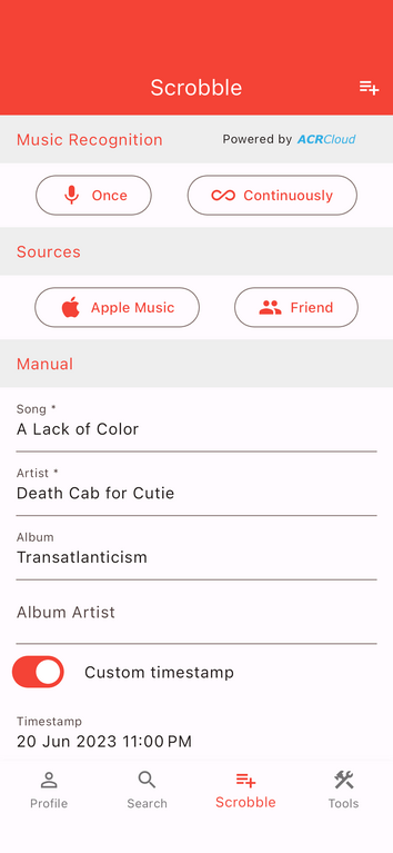
Almost a year ago I linked to Finale which is an iOS app that listens to the music you're playing and auto-scrobbles to last.fm using song recognition methods similar to Shazam or SoundHound. It works decently well, but it requires two devices: your iOS device (which can't be playing music), and something playing music over speakers. With these limitations its utility is somewhat stunted.
Recently I discovered RadioX 5, which is a Mac OS internet radio streaming application that includes the ability to scrobble plays to last.fm. It has many other features but this one is key for me. It lives in the menubar so it's very unobtrusive. The one disappointment is that it doesn't automatically scrobble songs — you need to manually hit the red circular last.fm icon in the app to save the play. At first this seems like a a huge omission, but without some external way of knowing what is a song and isn't, the application would end up scrobbling non-songs. For example, below is what the application shows when the DJ is speaking between songs on The Colorado Sound (I don't know why the cover art is for Lynyrd Skynyrd, it wasn't played before or after the DJ interlude). I wouldn't want to scrobble the non-song "The Colorado Sound" by the non-artist "The Colorado Sound."

Short of access to a comprehensive database of global artists+songs titles, which if it exists I'll bet wouldn't be cheap for programmatic use, I can think of one way that might allow for auto-scrobbling. If the application had a way to prevent scrobbling for a particular artist+song combination set by the user, probably custom to each radio station, then auto-scrobbling everything else might be practical.
more ...Infinite Mac
Sometime in 1994 me and my father went to a small computer show in the UC Berkeley Student Union building (which appears to now be named The MLK Jr. Building). It was probably a Macintosh oriented event, and among the various tables there was a Power Macintosh 6100 on display. The first Macintosh computers used Motorola 68000 series chips, and in 1994 Apple was making a transition to PowerPC chips. The 6100 was the first Mac to use a PowerPC chip, and seeing one in person was exciting. PowerPC chips promised a leap in performance, and I wanted one very badly. I had to wait at least a year to enter the PowerPC world when my father bought a PowerMac 8500.
Some time ago a Mac enthusiast released a website, Infinte Mac, that allows you to run old Mac operating systems in your browser. It starts with System 1.0, and has many releases all the way up to MacOS 9, the last version of the original Macintosh OS before they made the switch to the Unix-based OS that's still in use today. I suggest you try it out, it's really fun! I like playing with the various options because it reminds me of using and playing with computers from my childhood. The machines include quite a bit of pre-installed software. Many of the games I played actually work, which is impressive. It also shows how interfaces have evolved and mostly improved over the last 30-40 years.
The website uses various software emulators (including Basilisk II and SheepShaver) to simulate specific CPUs. To rephrase, what's happening is that the classic Macintosh system is running inside of a bit of software that, on the fly, translates old CPU instructions so that they run on a different CPU type. This is naturally less efficient than running instructions directly on a real CPU.
Recently I tried running a benchmark program (Macbench) in the emulator. Below is what I got on my M1 Max MacBook Pro. As you can see, the processor score is nearly five times faster than the PowerMac 6100 I wanted so long ago. Considering that my laptop has ten cores, my laptop is roughly 50 times faster than the PowerMac 6100 while running in emulated mode. It's been 30 years and of course progress progresses, but I still find it super impressive how much faster my laptop is using software emulation. Sitting here on my lap is a machine that's orders of magnitude better than what my 14 year old self wanted so badly. Huzzah!
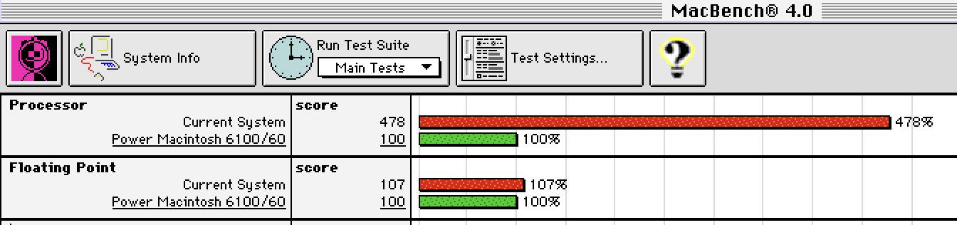
Earlier this month I bought a Mac Mini M4 to replace our six year old Mac Mini i3. As you can see, the M4 is over seven times faster than the PowerMac 6100. Being three generations newer than my laptop, it naturally gets a better score.

As an aside, I think that the floating point functions must be emulated in a less efficient way than the main processor functions. I don't think that the relatively low floating point scores are representative of the actual M1/M4 CPU performance.
more ...Setting Hadoop Node Types on AWS EMR
Amazon Web Services (AWS) offers dozens (if not over one hundred) different services. I probably use about a dozen of them regularly, including Elastic Map Reduce (EMR) which is their platform for running big-data things like Hadoop and Spark.
EMR runs your work on EC2 instances, and you can pick which kind(s) you want when the job starts. You can also pick the "lifecycle" of these instances. This means you can pick some instances to run as "on-demand" where the instance is yours (barring a hardware failure), and other instances to run as "spot" which costs much less than on-demand but AWS can take away the instance at any time.
Luckily, Hadoop and Spark are designed to work on unreliable hardware, and if previously done work is unavailable (e.g. because the instance that did it is no longer running), Hadoop and Spark can re-run that work again. This means that you can use a mix of on-demand and spot instances that, as long as AWS doesn't take away too many spot instances, will run the job for lower cost than otherwise.
A big issue with running Hadoop on spot instances is that multi-stage Hadoop jobs save some data between stages that can't be redone. This data is stored in HDFS, which is where Hadoop stores (semi)permanent data. Because we don't want this data going away, we need to run HDFS on on-demand instances, and not run it on spot instances. Hadoop handles this by having two kind of "worker" instances: "CORE" instances that run HDFS and have the important data, and "TASK" types that do not run HDFS and store easily reproduced data. Both types share in the computational workload, the difference is what kind of data is allowed to be stored on them. It makes sense, then, to confine "TASK" instances to spot nodes.
The trick is to configure Hadoop such that the instances themselves know what kind of instance they are. Figuring this out was harder than it should have been because AWS EMR doesn't auto-configure nodes to work this way; the user needs to configure the job to do this including running scripts on the instances themselves.
I like to run my Hadoop jobs using mrjob which makes development and running Hadoop with Python easier. I assume that this can be done outside of mrjob, but its up to the reader to figure out how to do that.
There are three parts to this. The first two are two Python scripts that are run on the EC2 instances, and the third is modifying the mrjob configuration file. The Python scripts should be uploaded to a S3 bucket because they will be downloaded to each Hadoop node (see the bootstrap actions below).
With the changes below, you should be able to run a multi-step Hadoop job on AWS EMR using spot nodes and not lose any intermediate work. Good luck!
make_node_labels.py
This script tells yarn what kind of instance types are available. This only needs to run once.
#!/usr/bin/python3
import subprocess
import time

def run(cmd):
    proc = subprocess.Popen(cmd,
        stdout = subprocess.PIPE,
        stderr = subprocess.PIPE,
    )
    stdout, stderr = proc.communicate()

    return proc.returncode, stdout, stderr

if __name__ == '__main__':

    # Wait for the yarn stuff to be installed
    code, out, err = run(['which', 'yarn'])
    while code == 1:
        time.sleep(5)
        code, out, err = run(['which', 'yarn'])

    # Now we wait for things to be configured
    time.sleep(60)

    # Now set the node label types
    code, out, err = run(["yarn",
        "rmadmin",
        "-addToClusterNodeLabels",
        '"CORE(exclusive=false),TASK(exclusive=false)"'])
get_node_label.py
This script tells Hadoop what kind of instance this is. It is called by Hadoop and run as many times as needed.
#!/usr/bin/python3
import json
k='/mnt/var/lib/info/extraInstanceData.json'
with open(k) as f:
    response = json.load(f)
    print("NODE_PARTITION:", response['instanceRole'].upper())
mrjob.conf
This is not a complete mrjob configuration file. It shows the essential parts needed for setting up CORE/TASK nodes. You will need to fill in the rest for your specific situation.
runners:
  emr:

    instance_fleets:
    - InstanceFleetType: MASTER
      TargetOnDemandCapacity: 1
      InstanceTypeConfigs:
      - InstanceType: (smallish instance type)
        WeightedCapacity: 1
    - InstanceFleetType: CORE
      # Some nodes are launched on-demand which prevents the whole job from
      # dying if spot nodes are yanked
      TargetOnDemandCapacity: NNN (count of on-demand cores)
      InstanceTypeConfigs:
      - InstanceType: (bigger instance type)
        BidPriceAsPercentageOfOnDemandPrice: 100
        WeightedCapacity: (core count per instance)
    - InstanceFleetType: TASK
      # TASK means no HDFS is stored so loss of a node won't lose data
      # that can't be recovered relatively easily
      TargetOnDemandCapacity: 0
      TargetSpotCapacity: MMM (count of spot cores)
      LaunchSpecifications:
        SpotSpecification:
          TimeoutDurationMinutes: 60
          TimeoutAction: SWITCH_TO_ON_DEMAND
      InstanceTypeConfigs:
      - InstanceType: (bigger instance type)
        BidPriceAsPercentageOfOnDemandPrice: 100
        WeightedCapacity: (core count per instance)
      - InstanceType: (alternative instance type)
        BidPriceAsPercentageOfOnDemandPrice: 100
        WeightedCapacity: (core count per instance)

    bootstrap:
    # Download the Python scripts to the instance
    - /usr/bin/aws s3 cp s3://bucket/get_node_label.py /home/hadoop/
    - chmod a+x /home/hadoop/get_node_label.py
    - /usr/bin/aws s3 cp s3://bucket/make_node_labels.py /home/hadoop/
    - chmod a+x /home/hadoop/make_node_labels.py
    # nohup runs this until it quits on its own
    - nohup /home/hadoop/make_node_labels.py &

    emr_configurations:
      - Classification: yarn-site
        Properties:
          yarn.node-labels.enabled: true
          yarn.node-labels.am.default-node-label-expression: CORE
          yarn.node-labels.configuration-type: distributed
          yarn.nodemanager.node-labels.provider: script
          yarn.nodemanager.node-labels.provider.script.path: /home/hadoop/get_node_label.py
Finale for last.fm
Since 2006 I've engaged in a bit of navel-gazing and tracked my music listening using last.fm. By running an application on your computer or phone, or linking a streaming service to last.fm (e.g. Tidal and Spotify support this), the service keeps track of what songs you listen to. The act of recording a song listen is called a "scrobble." However, it's always kind of bugged me that you can't scrobble in all situations, like when listening to an internet radio station or terrestrial radio.
Recently I discovered the Finale app that does exactly this: it not only allows you to manually enter songs, it includes Shazam-like ability to listen to songs and identify them for you, and if you like, then scrobble the song. It has a "continuously listen" mode which despite the name means that once a minute it wakes up and listens for any new song you're listening to and scrobbles for you.
Somewhat related, I would like to recommend The Colorado Sound, a music radio station operated by a local NPR affiliate. It's as commercial-free as NPR is (limited to "supported by" messages) and has a very wide and eclectic selection of music. Using the Finale app while I listen to their internet stream allows me to keep track of what they're playing, and if I hear something I like, I can revisit that song/artist. You should check it out!
more ...Solar Water Monitoring Page
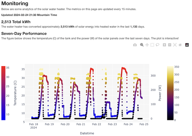
Today I just published a page that monitors my solar water heater. Every fifteen minutes the Raspberry Pi that controls the system pushes updated metrics to this website and triggers a refresh of the plots on the page. There's a diagram and description of how the whole system works. Go ahead and check it out!
more ...Bye Bye Bitbucket
A few days ago Bitbucket announced that they were ending support for Mercurial and will only support Git starting in about a year. I am a happy Mercurial user. It was the first DVCS system I learned, and have had no reason to switch away from it. Git is more popular than Mercurial, yes, but with useful plugins like hg-git, I never need to use Git even when I am working on a Git repository. Ultimately, the difference between Git and Mercurial is kind of like the difference between Windows and Mac (in that order). One is more popular than the other, but when it comes down to featureset and capabilities, it's very close. Like Windows vs. Mac, the main difference is the experience of using them, and I feel Mercurial is the clear winner.
I only use Bitbucket for their Mercurial support, so I decided to waste no time and abandon them entirely and immediately. In their place I am self-hosting an install of the community (open source) edition of Rhodecode. There are a couple of my repositories publicly viewable here. So far it seems like it has more than enough features to replace Bitbucket.
Update: As of this writing, I turned my self-hosted code server off because I'm lazy.
I feel I should point out that this serves as a reminder to me (and to you, dear reader) that cloud services cannot be relied upon. Companies, even if you are paying them, can stop serving you. This is at least the second time I have had to replace a cloud service with a self-hosted solution. A few years ago I replaced Google Reader with tt-rss. Like I wrote previously, because my new Mercurial hosting service is self-hosted, no one will be taking it away from me. And that is good.
Finally, I don't know why anyone would choose Bitbucket now to host their code repositories. Without Mercurial, all it has it Git, and Github (which has obviously been Git-only from the start) has already won:
more ...
State Fair Trip Planning
Some time ago I saw this blog post where Randal S. Olson used a genetic algorithm to compute an optimized path to visit various landmarks across the United States. I have used genetic algorithms professionally for a few things, and I found this application very fun and clever. As part of the blog post, Mr. Olson linked to the Jupyter notebook he used to calculate the optimized road trip. I am a heavy user of Python and the Jupyter notebook, so this intrigued me.
I got the idea to try to apply this kind thinking to the challenge to visiting the various state fairs that typically happen in the mid- to late-summer across the US. In fact, I got the idea to do this before the summer started. Indeed, some of the fairs analyzed below have already ended. But I have a good excuse! My second child was born very recently which has decreased my free time and increased the rate of brain cell death due to lack of sleep. These methods can be applied to future years by simply modifying the start/end dates where all the fairs are listed (in the notebook). Below are the results of my investigations.
The code behind these results can be found here.
Rules
- We only attend fairs in whole-day chunks. In reality, it's possible to arrive in town and attend the fair on the same day. But to keep this analysis simpler, we'll assume that travel days and fair attendance days are separate.
- We drive 12 hours a day. This is obviously something that comes down to personal preference, but I feel that 12 hours is fairly doable if you have more than one driver. Besides, who wants to attend all these fairs by themselves? What this rule means is that if it takes 12 hours and one second to get from point A to point B, the algorithm will count it as a two-day drive. This is obviously not realistic, but it keeps things simple.
When Do Fairs Happen?
Below is a Gantt chart that shows when the various fairs happen. The state name is on the y-axis, and time is on the x-axis. Except for Florida and Nevada, all the fairs happen in a fairly congested time frame between July and November.
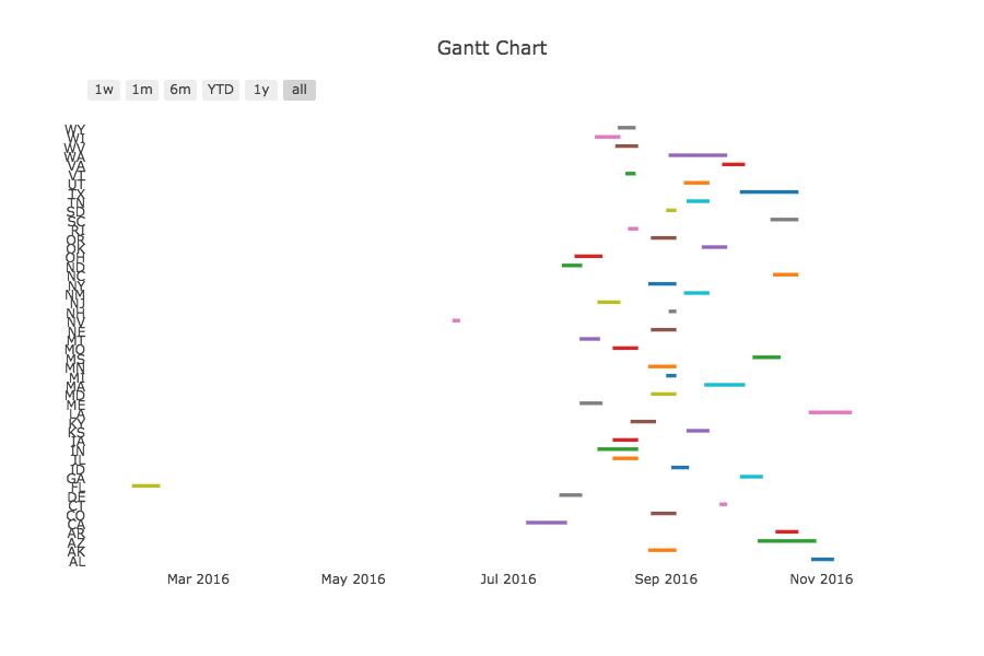
Quick note: As can be seen above, the Florida and Nevada state fairs take (took) place far earlier in the year than all the other fairs. Attending them doesn't conflict with any other fair, so I leave them out of my analyses until the end, or I just don't include them.
How to Spend the Most Days at a State Fair
I'm first going to answer question of how to spend the most days at a state fair in 2016. This is the way to eat the most fried things, ride the most rides, and see the most hog races in one summer. The winning strategy here is to get to a state fair and not leave it until you have to (e.g. it ends, or it's advantageous to leave for another fair), and also spend the least amount of time on the road between fairs.
For this analysis, we will not use a genetic algorithm, but rather a directional graph (digraph). This kind of graph is a network of nodes and edges, where the edges link nodes in an allowed direction of travel. In this case, the nodes will be fair attendance days, and the edges will be transitions. Some of the transitions will simply return to the same fair for consecutive attendance days, and other transitions will be travel to a new fair that cover one or more actual days.
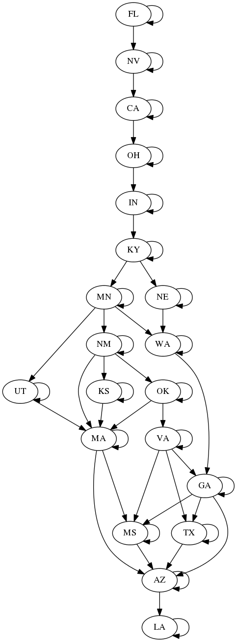
After a bunch of math and stuff (see the notebook!) we end up with 128 days that we can attend a fair. The diagram below describes the strategy of how to do this. Here's how to follow the diagram:
- Because they are temporally isolated, Florida and Nevada are to be attended first. We attend each fair for their full duration.
- Next we go to California. We see that there is an edge that goes back to California, and one that goes to Ohio. What this means is that we should stay in California as long as we can or want to, but we should travel directly to Ohio in time for that fair to be open.
- Likewise for Ohio and Indiana, we should stay at those fairs as long as we can/want to, and then travel to the next fair while it is still running.
- For Kentucky, after we have spent enough days there, we have an option of going to Minnesota or Nebraska. Whichever way we go here determines what fairs we can attend later on. For example, if we go to Nebraska, we can't go to New Mexico.
- Follow the rest of the the tree until we end up in Louisiana.
Most Days on the Road
What if you really like driving, but only if you have a destination? Are you some kind of weirdo? Let's see how we can attend state fairs all summer, but spend most of our time driving.
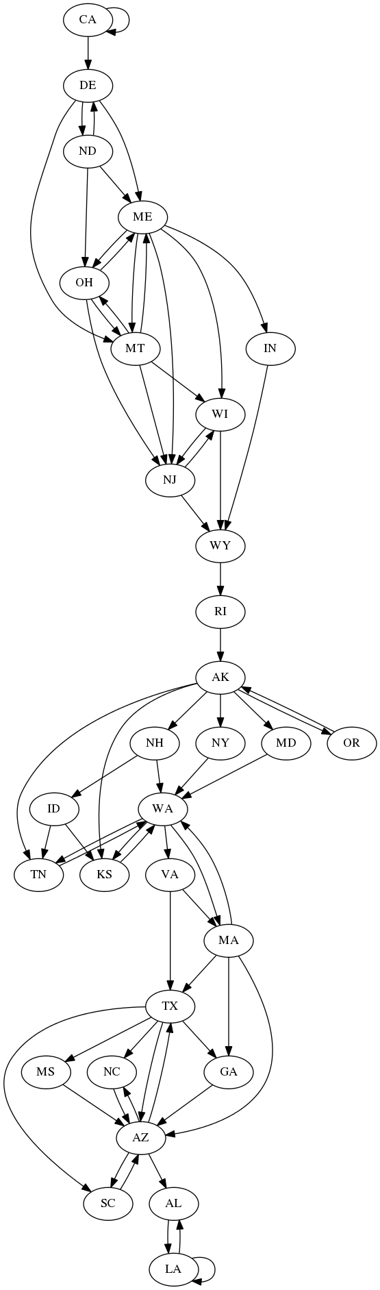
Doing some analysis similar to above, we come up with a method that puts us at state fairs for only 43 days. Note that I'm not including Florida nor Nevada in this count. This method has added 69 extra days of driving!
The strategy diagram below shows how to maximize driving time. It is quite a bit more complicated than the one above. It shows (as might be expected) that the optimal strategy here is to travel between distant fairs as much as possible, even going back and forth between fairs that are open at the same time. If you can travel to another fair far away, do it! For example, near the top there are links between Delaware and North Dakota going both ways. This means that to maximize traveling time, we should go to the Delaware fair, then North Dakota, and then return to Delaware again. After that we may travel back to North Dakota (if it's still open), or head over to Montana or Maine. Inspecting the diagram we'll notice some fair pairs that are very distantly separated (OR<->AK, WA<->TN), which again, makes sense if we are trying to maximize driving time. Also notice that out of the many possible paths, the WY->RI->AK segment is always the best strategy, which is hardly surprising, considering how long of a trip just those two segments are.
Whether or not this kind of strategy is a good idea is a very good question. But here it is. I dare anyone to try it!
Most Unique Fairs in One Summer (with the Lowest Driving Time)
This is the question of how to attend the most number of unique fairs in a single summer. What if we want to sample the character of as many fairs as possible? Which state fair has the best fried food? How might we go about that?
The work by Mr. Olson that inspired me to play around with state fairs used a genetic algorithm to determine a fairly efficient way to visit landmarks across the US. After much thought, I decided that a genetic algorithm would not work (easily) for this question. The reason is that the algorithm does various mutations, substitutions, and combinations that would be difficult to implement when time-ordered events limit choices.
For example, let's say we have a short segment in our path:
CA->DE->OH
and the genetic algorithm randomly decides to modify the Delaware step to a new fair. It can't just pick any fair because the new fair has to be open around the time the California fair. The new fair also has to be located such that we can travel to Ohio afterwards. Chances are that most new fair modifications wouldn't work at all.
Maybe the algorithm could replace the Delaware fair with a fair that works for California, but not Ohio. Then randomly picks the next fair (or fairs) replacing Ohio (and ones after that), fixing the chain until there's no more conflict. To me, that is not much different from just brute-forcing the problem because this would effectively destroy any genomes in the individual, and it would likely reduce its fitness.
This problem is probably as hard as the Traveling Salesman Problem. There are some differences between our problem here and the TSP, but my gut tells me that the two problems are similarly difficult:
- We do not need to visit all the possible states. For example, it's reasonable to expect that visiting Alaska will be very unlikely in any route that optimizes the number of unique fairs visited due to its prohibitive travel time.
- It's okay to visit a state fair more than once, most likely on consecutive days, but there's no rule that prevents us from coming back later if there are no other fairs we haven't already visited. This is a good thing, it means more fried food!
- Fairs are strictly ordered, which limits our available choices at any given time. It also requires us to visit a fair at a certain time which might limit some other options we might have pursued further down the line.
As daunting as this all sounds, a partially-random brute force method is easy to implement. Running it for five minutes gives us this recommended schedule below (in "State + Date" format) that results in visiting 38 state fairs (or 40 if we throw in Florida and Nevada). There's no guarantee that 40 states is the most that we can travel to in one calendar year, only a comprehensive search can prove that (which is a very, very expensive problem to solve). However, considering the size of our nation, and that there are two fairs that are impractical to attend (Alaska and Hawaii), and one that doesn't exist (Pennsylvania), 40/47 isn't bad at all.
'CA+2016-07-16',
 'DE+2016-07-21',
 'ND+2016-07-25',
 'OH+2016-07-28',
 'MT+2016-08-01',
 'WI+2016-08-04',
 'ME+2016-08-07',
 'NJ+2016-08-09',
 'MO+2016-08-12',
 'IL+2016-08-14',
 'WY+2016-08-17',
 'IA+2016-08-19',
 'IN+2016-08-21',
 'KY+2016-08-23',
 'NY+2016-08-25',
 'MN+2016-08-28',
 'NE+2016-08-30',
 'CO+2016-09-01',
 'OR+2016-09-04',
 'WA+2016-09-06',
 'ID+2016-09-08',
 'UT+2016-09-10',
 'NM+2016-09-12',
 'TN+2016-09-15',
 'KS+2016-09-17',
 'MA+2016-09-20',
 'CT+2016-09-22',
 'OK+2016-09-25',
 'VA+2016-09-28',
 'GA+2016-09-30',
 'TX+2016-10-02',
 'GA+2016-10-04',
 'MS+2016-10-06',
 'AZ+2016-10-09',
 'NC+2016-10-13',
 'SC+2016-10-15',
 'AR+2016-10-17',
 'AZ+2016-10-20',
 'AZ+2016-10-21',
 'AZ+2016-10-22',
 'AZ+2016-10-23',
 'AZ+2016-10-24',
 'LA+2016-10-27',
 'AL+2016-10-29 '
Anything Else?
Please leave a comment or send me a note (my email is easy to find) with any ideas.
more ...The Closest Non-Intersecting US Interstates
On our recent driving trip to Yellowstone and Montana, I had lots of time to think about random things while behind the wheel. One of them was to wonder of the major US Interstates, which two come the closest without actually intersecting? My guess was that it's some place on the East Coast, but due to my general lack of knowledge of East Coast highways, I had no idea which two it is.
Being a huge dork, I decided to figure it out.
Basically, it's actually not a very difficult thing to figure out. The steps are:
- Get the latitude and longitude coordinates for a number of points along each of the interstates.
- Determine which interstates intersect and eliminate those pairs.
- Put the coordinates for the interstates into a kD-Tree which will perform the search that determines the distance between non-intersecting highways in a fast way.
It turns out that the first step proved to be the hardest. I decided to use the data from the Open Street Map (OSM) project. This is a Google Maps-like website that is editable by anyone in the world, similar to Wikipedia. It will not give you directions like other mapping services, but it contains the geographical location of a wide variety of items, including and importantly (as the name suggests) roads. I looked into using the OSM APIs, but as far as I could tell either the APIs didn't do what I needed in an efficient way, or the servers were down. So I simply downloaded the 82 GB XML (5 GB compressed for download) dataset for the United States.
Begin rant feel free to skip to the next paragraph. I loathe XML. Any time that you have a 82 GB text file (apparently it's 200+ GB for the whole world) as your main distribution method, you're doing something wrong. Doing this project I learned as little about XML as I could to get just what I needed out of the file. Apparently the authoritative data is kept in a real database, but it appears that you can not download the data as a database. They do have a binary format description, but I can't find a link to download the data in that format. Furthermore, the world doesn't need yet another binary format. For example, they do not discuss endianness for their binary format on that wiki page, which is a big issue with binary formats. There are many other quality formats they could use (SQLite or HDF5). The binary format has a distinct Not Invented Here feel to it, which is nearly always a bad thing. Anyway, back to the main point of my rant. I don't care that the 82 GB XML file compresses down to 5 GB. Reading a 82 GB text file when you're searching for just a fraction of that data takes a long, long time, and is completely unnecessary. Every time I encounter XML it wastes my time in myriad ways. This time was no different. End rant
I'll spare you the full details and samples my low-quality Python code, but I munged the interstate data into a SQLite file, which distilled the data from 82 GB to 19 MB. Yes, that's nearly four orders of magnitude smaller. Then I used the much more convenient (and fast) SQLite file to build lists of interstate coordinates, which were fed into the kD-Tree for the nearest neighbor searches. The results are shown below. Note that there is no I-50 or I-60, and I eliminated I-45 from consideration because it's entirely within Texas, and therefore is not "major" in my opinion. I eliminated Hawaii's H-1 for the same reason. I have included links to maps showing the great circle between the nearest points of the highways. For highways that intersect, the link goes to one of the (more or less random) points of intersection.
Finally, we can see the answer I was looking for. Interstates 70 and 95 come within 5 kilometers in Baltimore at the terminus of 70, but do not intersect. So my suspicion was correct that it was somewhere in the East, so I have that to feel good about.
| X | 95 | 90 | 85 | 80 | 75 | 70 | 65 | 55 | 40 | 35 | 30 | 25 | 20 | 15 | 10 |
| 5 | 3338 | 2877 | 2826 | 690 | 2741 | 2484 | 142 | 1760 | 1822 | 910 | 1237 | ||||
| 10 | 1195 | 178 | 544 | 558 | 91 | 321 | |||||||||
| 15 | 2860 | 2423 | 2029 | 2009 | 1839 | 1272 | 1489 | 436 | 1093 | ||||||
| 20 | 804 | 764 | 615 | 173 | 283 | ||||||||||
| 25 | 2185 | 1730 | 1653 | 1453 | 1239 | 629 | 749 | ||||||||
| 30 | 1062 | 865 | 610 | 758 | 643 | 458 | 486 | 191 | |||||||
| 35 | 1404 | 985 | 569 | 516 | 358 | ||||||||||
| 40 | 587 | 550 | 347 | ||||||||||||
| 55 | 806 | 340 | 319 | 37 | |||||||||||
| 65 | 465 | 101 | |||||||||||||
| 70 | 5 | 152 | 234 | 105 | |||||||||||
| 75 | 12 | ||||||||||||||
| 80 | 413 | ||||||||||||||
| 85 | 582 | ||||||||||||||
| 90 |
p.s. If you really, really want to see the code I used for this, I can share it, but I'll have to pull out the hamsters that have taken residence in it. They're attracted to dusty littered places, you know.
more ...SciPy 2009 at Caltech
I'm at the SciPy 2009 conference at Caltech in Pasadena today and yesterday. It is an amazing collection of nerds and questionable facial hair styles. There have been some interesting talks.
I like this "snub cube" fountain:

The SciPy crowd:
A fountain in front of the building the conference is in:

New Hosting Service, Again
Two and a half years ago I moved my website off my father's computer at home to Site5. For a while it was great, especially compared to serving a website over a cable modem connection. However, over the last year or two it's gotten progressively worse, something I discussed in this post about a year ago. Also over a year ago, Site5 promised to move everyone to new servers. It hasn't happened, and my service has gone steadily downhill.
My first two-year prepaid period with Site5 went up in December last year, and I seriously thought about moving. I looked at other shared hosting companies, but I felt I would probably have the same problems on a new shared host. I looked into hybrid solutions, but that too didn't seem a guaranteed improvement. I liked the idea of Virtual Private Servers (VPS), but I couldn't find one with enough disk space in my budget.
A few months ago, my lab mate Rick pointed me towards s3fs, which intrigued me. s3fs puts your data on Amazon S3, but allows the data to appear to be local to the server, like another hard drive. You pay for only what you use with S3, and it has virtually unlimited space. Suddenly, a VPS hosting solution fit into my budget. I could pay for a VPS with less disk space than I needed, but still get the power of VPS. It was also an upgrade because now me and my family could upload as much data as we wanted, and it would be much more secure from disk failure than before.
This website and other sites that were on the old server are now being hosted on a machine from linode.com. I'm using their lowest option, which has 10GB of space. I installed Ubuntu Hardy Heron which seems like a solid Linux distribution. s3fs has proven to be reliable and fast enough, although it's much slower than having the data on a local disk. Using Apache rewrites, my father and I have made it such that when a web browser asks for items on a page that exists on S3, the request goes there instead from this server, which saves lots of time. I've also figured out how to shoehorn Gallery2 into using S3.
So far I am very happy with the new server.
more ...Yahoo! Mail Tries, and Misses
I have written thrice (1, 2, 3) in the past about the new Yahoo! mail interface, the Ajaxed interface to Yahoo! mail. It is incredible how slowly they make improvements to it. It's not like Yahoo! cares what I say, but of the points I raised over two years ago in my first post, they still haven't all been fixed.
But Yahoo! maybe trying harder. There is now a preference to add the greater-than signs on replied to messages:

Which is great. Until you try to use it. Here is a message I sent myself:
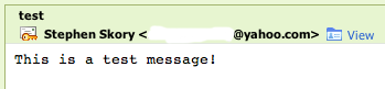
Here is what I get when I hit "reply" (this is a screen shot of the compose window, the text is editable):
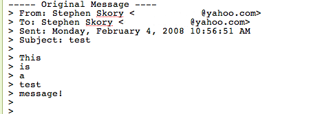
Yes, each and every word of the message I'm replying to gets its own line. But it gets worse! Here's what I get when I send the replied message without touching anything:
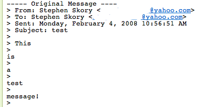
Here each word of the replied to message gets its own line separate from the greater-than signs. I hope this is just a simple bug (I will submit a bug report about this) but this is simply ridiculous.
more ...Yahoo! Mail Beta still stinks… less
Three months ago I wrote that Yahoo! Mail Beta still stinks. I said that Yahoo! had fixed two of my five main quibbles with their newest email interface. Sure, they fixed two, but they were the ones I cared least about.
Lo and behold, Yahoo! came out with an updated version of Mail Beta a month ago, and more recently my server farm received the update. Let's see how Yahoo! fares this round!
-
Fixed-width fonts. Huzzah! Numbah one gets addressed. This is big. Fixing this almost is enough for me to start using Beta every day. But only almost. Yahoo!, you get a nice green check:

-
Message replying format. Nope. Nothing new here. Same, lame behavior as before. Give us some freedom, Yahoo!. Stop putting the minority with good etiquette down! This earns you a Big Red X, and red is never a good color for anything.

-
Message quoting. Nope, again. There is still no way to differentiate the message I'm replying to and what I've written. Another BRX.
Yahoo!, you're getting beat up, down, left and right by Google. They just took YouTube out from under you this week! Shape up!
more ...