How I Got a 327x Speedup Of Some Python Code
I don't usually post code stuff on this blog, but I had some fun working on this and I wanted to share!
My colleague, Abhi, is processing data from an instrument collecting actual data from the real world (you should know that this is something I have never done!) and is having some problems with how long his analysis is taking. In particular, it is taking him longer than a day to analyze a day's worth of data, which is clearly an unacceptable rate of progress. One step in his analysis is to take the data from all ~30,000 frequency channels of the instrument, and calculate an average across a moving window 1,000 entries long. For example, if I had the list:
[0, 1, 2, 3, 4, 5, 6, 7, 8, 9]
and I wanted to find the average over a window of length three, I'd get:
[1, 2, 3, 4, 5, 6, 7, 8]
Notice that I started by averaging [0, 1, 2]=>1, as this is the first way to come up with a window of three values. Similarly, the last entry is [7, 8, 9]=>8. Here is a simplified version of how Ahbi was doing it (all of the code snippets shown here are also available [here][1]):
def avg0(arr, l):
    # arr - the list of values
    # l - the length of the window to average over
    new = []
    for i in range(arr.size - l + 1):
        s = 0
        for j in range(i, l + i):
            s += j
        new.append(s / l)
    return new
This function is correct, but when we time this simple function (using an IPython Magic) we get:
# a is [0, 1, 2, ..., 29997, 29998, 29999]
a = np.arange(30000)
%timeit avg0(a, 1000)
1 loops, best of 3: 3.19 s per loop
Which isn't so horrible in the absolute sense -- 3 seconds isn't that long compared to how much time we all waste per day. However, I neglected to mention above that Abhi must do this averaging for nearly 9,000 chunks of data per collecting day. This means that this averaging step alone takes about 8 hours of processing time per day of collected data. This is clearly taking too long!
The next thing I tried is to take advantage of Numpy, which is a Python package that enables much faster numerical analysis than with vanilla Python. In this function I'm essentially doing the same thing as above, but using Numpy methods, including pre-allocating space, summing values using the accelerated Numpy .sum() function, and using the xrange() iterator, which is somewhat faster than plain range():
def avg1(arr, l):
    new = np.empty(arr.size - l + 1, dtype=arr.dtype)
    for i in xrange(arr.size - l + 1):
        new[i] = arr[i:l+i].sum() / l
    return new
This provides a healthy speed up of about a factor of eight:
%timeit avg1(a, 1000)
1 loops, best of 3: 405 ms per loop
But this still isn't fast enough; we've gone from 8 hours to just under an hour. We'd like to run this analysis in at most a few minutes. Below is an improved method that takes advantage of a queue, which is a programming construct that allows you to efficiently keep track of values you've seen before.
def avg2(arr, l):
    new = np.empty(arr.size - l + 1, dtype=arr.dtype)
    d = deque()
    s = 0
    i = 0
    for value in arr:
        d.append(value)
        s += value
        if len(d) == l:
            new[i] = s / l
            i += 1
        elif len(d) > l:
            s -= d.popleft()
            new[i] = s / l
            i += 1
    return new
And here we can see that we've cut our time down by another factor of 4:
%timeit avg2(a, 1000)
10 loops, best of 3: 114 ms per loop
This means that from 8 hours we're now down to roughly 13 minutes. Getting better, but still not great. What else can we try? I've been looking for an excuse to try out Numba, which is a tool that is supposed to help speed up numerical analysis in Python, so I decided to give it a shot. What makes Numba attractive is that with a single additional line, Numba can take a function and dramatically speed it up by seamlessly converting it into C and compiling it when needed. So let's try this on the first averaging function:
@jit(argtypes=[int32[:], int32], restype=int32[:])
def avg0_numba(arr, l):
    new = []
    for i in range(arr.size - l + 1):
        s = 0
        for j in range(i, l + i):
            s += j
        new.append(s / l)
    return np.array(new)
In the line beginning with @jit, all I have to do is describe the input and the output types, and it handles the rest. And here's the result:
%timeit avg0_numba(a, 1000)
10 loops, best of 3: 21.6 ms per loop
What is incredible here is that not only is this roughly 5 times faster than the queue method above, it's a ridiculous 147 times faster than the original method and only one line has been added. We've now reduced 8 hours to about 4 minutes. Not bad!
Let's try this on the second averaging method, which if you recall, was substantially better than the original method:
@jit(argtypes=[int32[:], int32], restype=int32[:])
def avg1_numba(arr, l):
    new = np.empty(arr.size - l + 1, dtype=arr.dtype)
    for i in xrange(arr.size - l + 1):
        new[i] = arr[i:l+i].sum() / l
    return new
%timeit avg1_numba(a, 1000)
1 loops, best of 3: 688 ms per loop
That's interesting! For some reason I don't understand, this is actually slower than the un-optimized version of avg1. Let's see if Numba can speed up the queue method:
@jit(argtypes=[int32[:], int32], restype=int32[:])
def avg2_numba(arr, l):
    new = np.empty(arr.size - l + 1, dtype=arr.dtype)
    d = deque()
    s = 0
    i = 0
    for value in arr:
        d.append(value)
        s += value
        if len(d) == l:
            new[i] = s / l
            i += 1
        elif len(d) > l:
            s -= d.popleft()
            new[i] = s / l
            i += 1
    return new
%timeit avg2_numba(a, 1000)
10 loops, best of 3: 77.5 ms per loop
This is somewhat better than before, but still not as fast as avg0_numba, which comes in at roughly 20ms. But what if I really try hard to optimize the queue method by using only Numpy arrays?
@jit(argtypes=[int32[:], int32], restype=int32[:])
def avg2_numba2(arr, l):
    new = np.empty(arr.size - l + 1, dtype=arr.dtype)
    d = np.empty(l + 1, dtype=arr.dtype)
    s = 0
    i = 0
    left = 0
    right = 0
    full = False
    for j in xrange(arr.size):
        d[right] = arr[j]
        s += arr[j]
        right = (right + 1) % (l+1)
        if not full and right == l:
            new[i] = s / l
            i += 1
            full = True
        elif full:
            s -= d[left]
            left = (left + 1) % (l+1)
            new[i] = s / l
            i += 1
    return new
%timeit avg2_numba2(a, 1000)
100 loops, best of 3: 9.77 ms per loop
A ha! That's even faster, and our 3.19s are now down to 9.77ms, an improvement of 327 times. The original 8 hours are now reduced to less than two minutes. I hope you've enjoyed this as much as I have!
Update:
After chatting with a couple of my colleagues, this appears to be the fastest way to do this kind of operation:
from scipy.signal import fftconvolve
import numpy as np
a = np.arange(30000)
b = np.ones(1000) / 1000.
%timeit fftconvolve(a, b, 'valid')
100 loops, best of 3: 6.25 ms per loop
Working Conditions
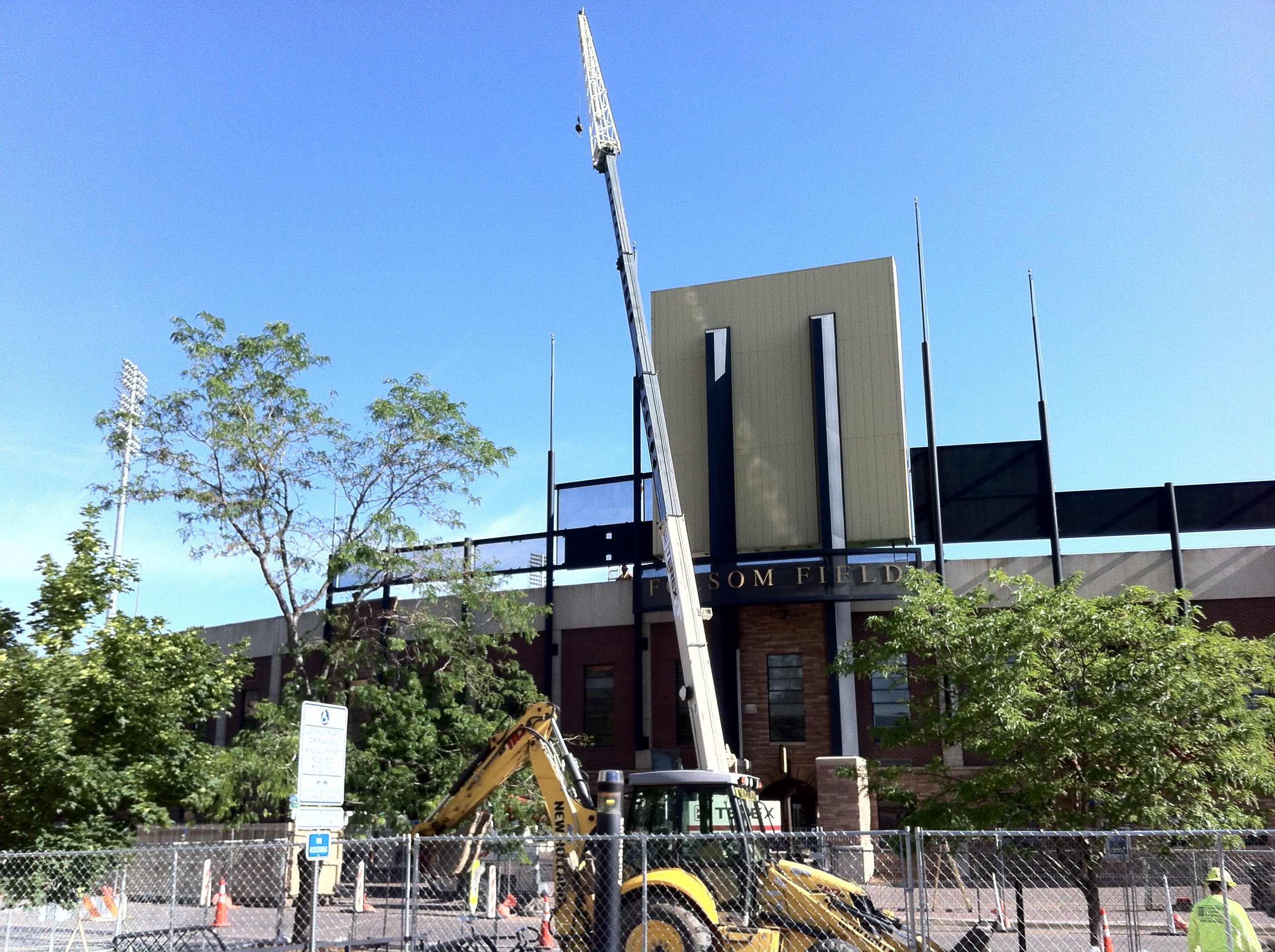
Of late, there has been a great deal of construction in and around my office. Beginning two weeks ago my office cluster has been repainted, doors refinished, window shades replaced, some carpet has been replaced, and some wires and pipes have been installed and moved. There is still some more work to be done.
Beginning yesterday, and continuing for the next four to six weeks, the scoreboards for the stadium are being replaced. Pictured above is a crane removing pieces of the old one (notice the asymmetry in solid black/shaded regions). This crane is more or less just outside my window, which, as you can imagine, is kind of neat for the first five minutes, and then gets tiresome and annoying after that. The construction has also closed off large amount of space in front of the offices which is inconvenient for us, and they even cut down two perfectly healthy trees, presumably to make space for the crane (insert tree-sitter joke here).
As a matter of fact, the conduit carrying the control wires for the new scoreboards passes by my office. The next time Stanfurd plays the Buffs, don't be surprised if - wait, I'm saying too much.
more ...CU Janus Supercomputer
Last night I had the opportunity to tour the supercomputer recently built here at CU named "Janus" that I've been using. It is a 16,000-core Dell cluster using 6-core Intel processors running RedHat Linux. It was built in an interesting way. Instead of building a machine room in a building and then filling it with cooling ducts, pipes, and power connections, the machine room is made up of standard shipping containers that had all those connections in place, similar to a pre-fab house. These were shipped from the factory (in Canada, I think) on trucks, and then dropped next to each other in a parking lot behind a campus building. Unfortunately, because it was nighttime, I don't have a good picture of the outside.
Below are some pictures I took of Janus.

The machine racks. The door encloses the 'hot' side of the machines, where the air is sucked to the heat exchangers.
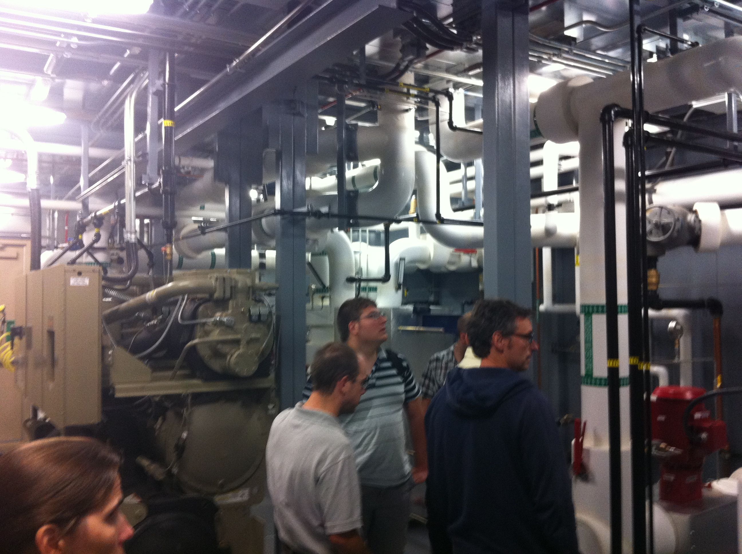
The cooling system.

The blinky and hot end of the machines. Lots of wires!
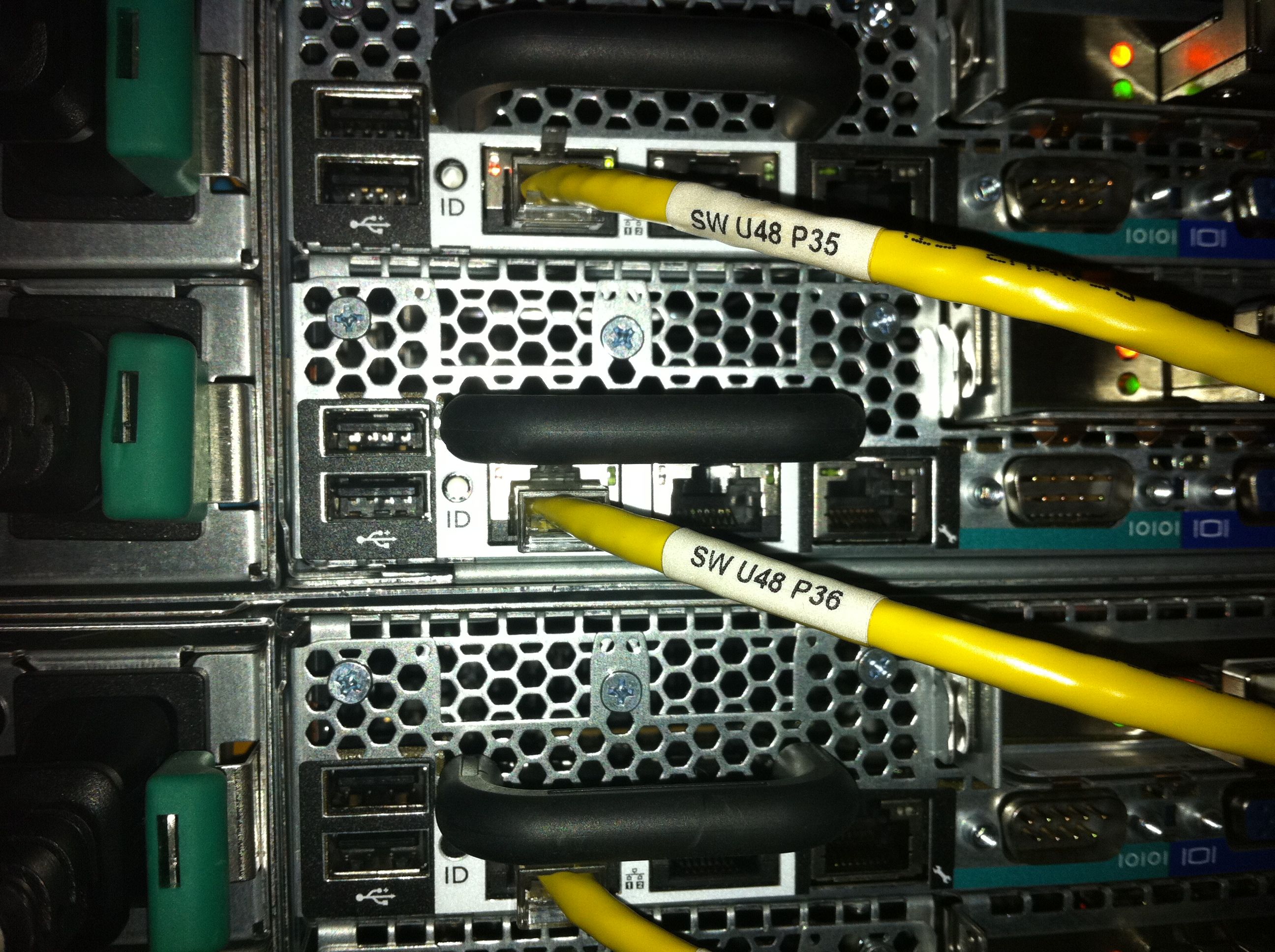
A close up of the back of a compute node. Notice that they have serial ports, which are based on a 40+ year old standard. At least they have USB ports, too.
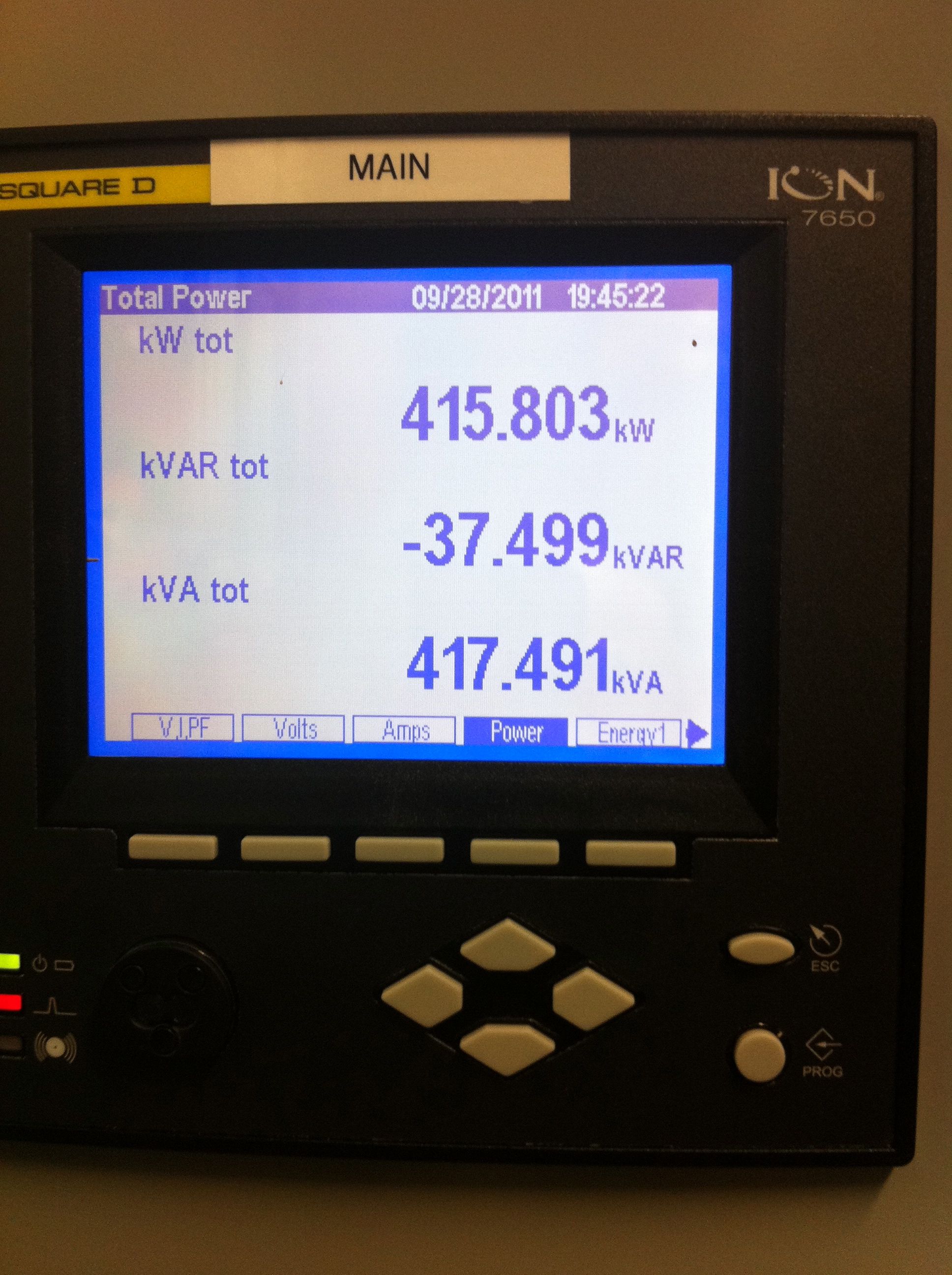
It was using 415 kW of power. I think it can go much higher than that when the machine is under heavy load on a hot day.
more ...Blob Identification
I have access to some of the fastest computers in the world. I can summon thousands of processors, petabytes of disk storage, and terabytes of memory with a few keystrokes. You'd think with that kind of power, analysis could be automated and done in massive pipelines. But that's not always true. Sometimes things are so subtle that the most efficient method is still to use the human eye.
Today I was pretty ill, with a sore throat and congestion. It was the kind of day for lying on the couch and watching movies. Luckily, I was able to accomplish some work that didn't require too much concentration. First, some context.
One of my current projects is looking at the centers of simulated galaxy clusters, and it is actually surprisingly difficult to find the centers of the clusters. Clusters are complicated places, with clumps of matter falling in, sloshing stuff around, making the core not exactly clear. In order to semi-automate the process, I wrote a script that makes pictures of the clusters (which have been previously identified in a automated fashion), that have density contours superimposed. The density contours are analogous to the lines on a topographical map.
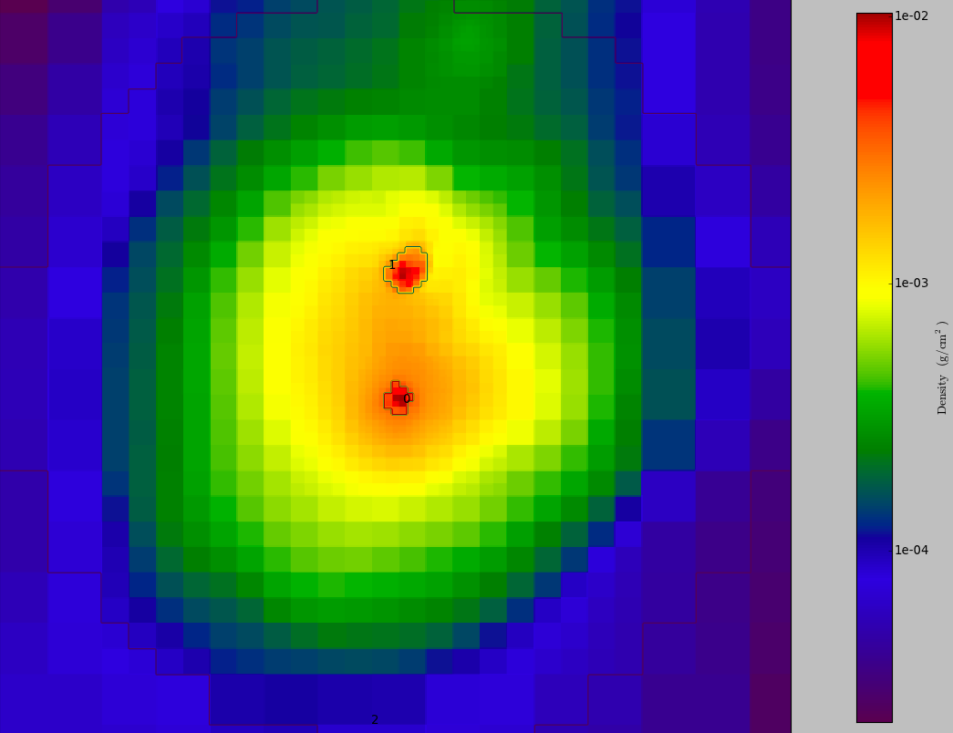
The picture above is an example of the output of the script. The colors indicate gas density, blue to red is low to high. If you look at the full-sized image, you can see that there are two dense clumps numbered 0 and 1. I can't just pick the most dense cluster because that might be a tiny blob of matter falling into the larger cluster; more care is needed. So I need to make the decision with my adaptable brain. The script spits out the image, and then I have to input which clump I think is the most central clump, and a record is made which I'll use for the next step in my chain of analysis. I spent most of today looking at these pictures and entering numbers. Yay for tax payers!
This is very similar to the Galaxy Zoo project that aimed to identify the morphology of actual galaxies, but my effort is on a much smaller and simpler scale.
So - which clump do you think is the most central above?
more ...Volume Rendered Movies
It's show-and-tell time! Below are two movies I made using the volume rendering tools of yt. I've been using yt for a few years to analyze and visualize the cosmological simulations I make with Enzo, and only recently have I had time to begin to play with the new volume rendering stuff.
The first movie is a slow rotation around the entire volume of a simulation at a contemporary epoch, which means that this image is produced from the state of simulation at its end, 13 billion years after it started. The colors correspond to the density of matter in the volume, from dark blue to white as density increases. The simulation is a periodic cube with dimensions 20 Mpc/h on a side. In comparison, the diameter of our galaxy is somewhere around one thousand times smaller. This means that the whitest areas correspond to clusters of galaxies, and our galaxy would be just a small part of one of the white blobs. Be sure to watch the movie full screen!
Below shows the time evolution of the simulation from beginning to end. This is a thin slab of the center of the simulation (10% thickness) viewed from a corner of the cube. Notice that early on the matter is very clumpy everywhere, but rapidly forms dense knots connected by thin filaments. This is how the real universe looks! After about the half-way point of the movie you'll notice that not much happens. Again, this is how the real universe looks! Much of the large-scale evolution of the universe was finished about 7 billion years ago. This movie uses comoving coordinates, that compensate for the expansion of the universe. If I were to use proper coordinates, which are the kind we use every day to measure normal things with rulers, the movie would show the simulation starting very small and then blowing up. Again, use the full screen option for the best image.
more ...
SDSC Optiportal
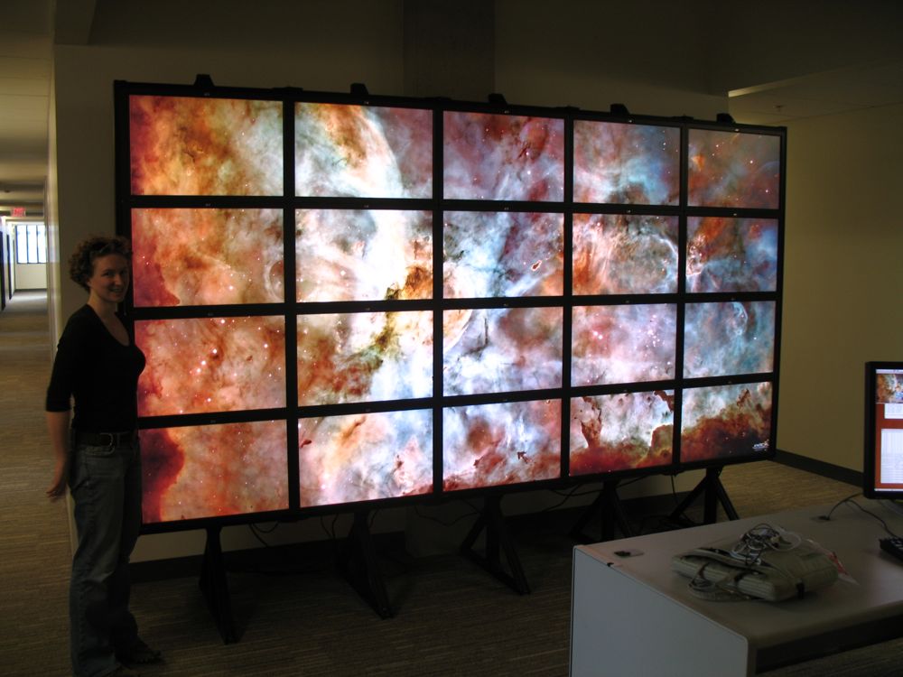
My adviser Professor Mike Norman, as part of his job at the San Diego Supercomputer Center, purchased an optiportal system for the new SDSC building which is opening today. An optiportal system is a wall of monitors powered by networked computers such that the screens behave as one monitor. Very high resolution images and movies can be tiled across the screens, as you can see below. Movies and animations can also be tiled across the screens.
My labmates and I (Rick Wagner in particular) spent the last week feverishly building the system. The primary work was to build the monitor rack. It has many bolts and sliders and adjustments. We arranged to have two holes drilled through the wall for the monitor cables. The 30-inch screens require a very particular kind of cable and getting enough of the right kind that were long enough to reach all the screens was surprisingly difficult.
My main task was to convert some of the publicly available high-resolution astronomical images into tiled TIFFs. Tiled TIFFs break the data up into easy to scale tiles, which is essential for the optiportal. I used many of the images from this page (link broken), including the 403 megapixel Carina Nebula image linked there. It was quite frustrating. I tried half a dozen computers and iterations of ImageMagick and VIPS before I finally got a combination that worked.
In some ways, this is worse than a projector. There are gaps between the screens. This requires multiple expensive computers and many, many cables. However, there are some big advantages to this setup. There is no projector that has anywhere the same resolution as this optiportal (2560x1600x20 = 81.92 megapixels). Just one of the monitors is better than all but the most specialized and expensive projectors. The screens are bright and clear, even in normal lighting conditions. Unlike a projector, standing in front of the screen doesn't shadow the image. It has to be seen for yourself; twenty 30-inch monitors are awesome to behold.
Each four-monitor column is powered by a HP xw8600 workstation with one 4-core 2.33GHz Xeon processor, 4GB of RAM, two NVIDIA Quadro FX4600 768MB video cards with dual output, running Ubuntu 8.04 LTS. There is a sixth identical workstation that serves as a head node which sits in front of the screens and controls the output on the wall. There is also a HP ML370 server that has a 1TB RAID5 disk array, and has room for an additional 1TB. Eventually, all the machines will be connected by a 10Gb CX-4 network using a ProCurve 6400cl-6XG switch, and the head node and disk server will be connected to the outside world with a 10Gb optical connection. The monitor array is controlled using CGLX which is developed at Calit2, which is here at UCSD.
Science will not be performed on the optiportal, at least the major calculations won't. Instead, visualizations of simulations run on supercomputers will be displayed and analyzed. The human eye and brain is still a superior judge of the accuracy and meaning of data than a set of conditional equations. It is often necessary to actually see the raw data as clearly as possible. The point of the eventual 10Gb optical connection is that various parallel visualization programs like VisIt and ParaView will be practical. These programs do the data analysis on a remote supercomputer and the visualization is sent to the optiportal in real time for display. In this way, terabytes of raw data don't have to be transferred off the supercomputer, and the computationally intensive part of the visualization takes place on the supercomputer, which has far more processors, RAM and disk space than the optiportal. I hope to someday have some of my data displayed in this fashion.
more ...Cray Coolness
I'm back on the new supercomputer in Tennessee: the Cray XT4 Kraken. The coolest command on the computer, in my opinion, is xtshowcabs. Below is the (anonymized) output. This shows which job is running on each node (each processor has four cores in one processor). The lower-case letters correspond to jobs listed at the bottom. Each vertical set of symbols (eight wide, twelve high) is a physical cabinet of nodes*.
What you see below is one job running 8192 cores (a), another running on 4096 (h), one with 2048 (k) and a smattering of smaller jobs. My jobs are i and j, running on 8 cores each. The computer is just about full here, about 96% usage.
This also allows me to know who to blame when my jobs are sitting waiting to start for days.
Compute Processor Allocation Status as of Fri Aug  1 18:14:16 2008

     C0-0     C0-1     C0-2     C0-3     C1-0     C1-1     C1-2     C1-3
  n3 -------- -------- hhhhhhhh hhhhhhhh SSSaaaaa aaaaaaaa aaaaaaaa aaaaaaak
  n2 -------- -------- hhhhhhhh hhhhhhhh    aaaaa aaaaaaaa aaaaaaaa aaaaaaak
  n1 -------- -------- hhhhhhhh hhhhhhhh    aaaaa aaaaaaaa aaaaaaaa aaaaaaak
c2n0 -------- -------- hhhhhhhh hhhhhhhh SSSaaaaa aaaaaaaa aaaaaaaa aaaaaaak
  n3 SSSSS--- -------- hhhhhhhh hhhhhhhh SSSSaaaa aaaaaaaa aaaaaaaa aaaaaaaa
  n2      --- -------- hhhhhhhh hhhhhhhh     aaaa aaaaaaaa aaaaaaaa aaaaaaaa
  n1      --- -------- hhhhhhhh hhhhhhhh     aaaa aaaaaaaa aaaaaaaa aaaaaaaa
c1n0 SSSSS--- -------- hhhhhhhh hhhhhhhh SSSSaaaa aaaaaaaa aaaaaaaa aaaaaaaa
  n3 SSSSSSSS -------- --lihhhh hhhhhhhh SSSSaaaa aaaaaaaa aaaaaaaa aaaaaaaa
  n2          -------- --ljhhhh hhhhhhhh     aaaa aaaaaaaa aaaaaaaa aaaaaaaa
  n1          -------- --ljhhhh hhhhhhhh     aaaa aaaaaaaa aaaaaaaa aaaaaaaa
c0n0 SSSSSSSS -------- ---lihhh hhhhhhhh SSSSaaaa aaaaaaaa aaaaaaaa aaaaaaaa
    s01234567 01234567 01234567 01234567 01234567 01234567 01234567 01234567

     C2-0     C2-1     C2-2     C2-3     C3-0     C3-1     C3-2     C3-3
  n3 hhhhhhhh hhhhhhhh hhhhhhhh hhhhhhhh aaaaaaaa aaaaaaaa aaaaaaaa aaaaaaaa
  n2 hhhhhhhh hhhhhhhh hhhhhhhh hhhhhhhh aaaaaaaa aaaaaaaa aaaaaaaa aaaaaaaa
  n1 hhhhhhhh hhhhhhhh hhhhhhhh hhhhhhhh aaaaaaaa aaaaaaaa aaaaaaaa aaaaaaaa
c2n0 hhhhhhhh hhhhhhhh hhhhhhhh hhhhhhhh aaaaaaaa aaaaaaaa aaaaaaaa aaaaaaaa
  n3 hhhhhhhh hhhhhhhh hhhhhhhh hhhhhhhh aaaaaaaa aaaaaaaa aaaaaaaa aaaaaaaa
  n2 hhhhhhhh hhhhhhhh hhhhhhhh hhhhhhhh aaaaaaaa aaaaaaaa aaaaaaaa aaaaaaaa
  n1 hhhhhhhh hhhhhhhh hhhhhhhh hhhhhhhh aaaaaaaa aaaaaaaa aaaaaaaa aaaaaaaa
c1n0 hhhhhhhh hhhhhhhh hhhhhhhh hhhhhhhh aaaaaaaa aaaaaaaa aaaaaaaa aaaaaaaa
  n3 hhhhhhhh hhhhhhhh hhhhhhhh hhhhhhhh aaaaaaaa aaaaaaaa aaaaaaaa aaaaaaaa
  n2 hhhhhhhh hhhhhhhh hhhhhhhh hhhhhhhh aaaaaaaa aaaaaaaa aaaaaaaa aaaaaaaa
  n1 hhhhhhhh hhhhhhhh hhhhhhhh hhhhhhhh aaaaaaaa aaaaaaaa aaaaaaaa aaaaaaaa
c0n0 hhhhhhhh hhhhhhhh hhhhhhhh hhhhhhhh aaaaaaaa aaaaaaaa aaaaaaaa aaaaaaaa
    s01234567 01234567 01234567 01234567 01234567 01234567 01234567 01234567

     C4-0     C4-1     C4-2     C4-3     C5-0     C5-1     C5-2     C5-3
  n3 hhhhhhhh hhhhhhhh hhhhhhhh hhhhhhhh aaaaaaaa aaaaaaaa aaaaaaaa aaaaaaaa
  n2 hhhhhhhh hhhhhhhh hhhhhhhh hhhhhhhh aaaaaaaa aaaaaaaa aaaaaaaa aaaaaaaa
  n1 hhhhhhhh hhhhhhhh hhhhhhhh hhhhhhhh aaaaaaaa aaaaaaaa aaaaaaaa aaaaaaaa
c2n0 hhhhhhhh hhhhhhhh hhhhhhhh hhhhhhhh aaaaaaaa aaaaaaaa aaaaaaaa aaaaaaaa
  n3 hhhhhhhh hhhhhhhh hhhhhhhh hhhhhhhh aaaaaaaa aaaaaaaa aaaaaaaa aaaaaaaa
  n2 hhhhhhhh hhhhhhhh hhhhhhhh hhhhhhhh aaaaaaaa aaaaaaaa aaaaaaaa aaaaaaaa
  n1 hhhhhhhh hhhhhhhh hhhhhhhh hhhhhhhh aaaaaaaa aaaaaaaa aaaaaaaa aaaaaaaa
c1n0 hhhhhhhh hhhhhhhh hhhhhhhh hhhhhhhh aaaaaaaa aaaaaaaa aaaaaaaa aaaaaaaa
  n3 hhhhhhhh hhhhhhhh hhhhhhhh hhhhhhhh aaaaaaaa aaaaaaaa aaaaaaaa aaaaaaaa
  n2 hhhhhhhh hhhhhhhh hhhhhhhh hhhhhhhh aaaaaaaa aaaaaaaa aaaaaaaa aaaaaaaa
  n1 hhhhhhhh hhhhhhhh hhhhhhhh hhhhhhhh aaaaaaaa aaaaaaaa aaaaaaaa aaaaaaaa
c0n0 hhhhhhhh hhhhhhhh hhhhhhhh hhhhhhhh aaaaaaaa aaaaaaaa aaaaaaaa aaaaaaaa
    s01234567 01234567 01234567 01234567 01234567 01234567 01234567 01234567

     C6-0     C6-1     C6-2     C6-3     C7-0     C7-1     C7-2     C7-3
  n3 hhhhcccc cccccccc bbbbbbbb gggggggg aaaaaaaa aaaaaaaa aaaaaaaa aaaaaaaa
  n2 hhhhcccc cccccccc bbbbbbbb gggggggg aaaaaaaa aaaaaaaa aaaaaaaa aaaaaaaa
  n1 hhhhcccc cccccccc bbbbbbbb gggggggg aaaaaaaa aaaaaaaa aaaaaaaa aaaaaaaa
c2n0 hhhhhccc cccccccc bbbbbbbb gggggggg aaaaaaaa aaaaaaaa aaaaaaaa aaaaaaaa
  n3 hhhhhhhh cccccccc bbbbbbbb bbbbgggg aaaaaaaa aaaaaaaa aaaaaaaa aaaaaaaa
  n2 hhhhhhhh cccccccc bbbbbbbb bbbbgggg aaaaaaaa aaaaaaaa aaaaaaaa aaaaaaaa
  n1 hhhhhhhh cccccccc bbbbbbbb bbbbgggg aaaaaaaa aaaaaaaa aaaaaaaa aaaaaaaa
c1n0 hhhhhhhh cccccccc bbbbbbbb bbbbbggg aaaaaaaa aaaaaaaa aaaaaaaa aaaaaaaa
  n3 hhhhhhhh cccccccc ccccbbbb bbbbbbbb aaaaaaaa aaaaaaaa aaaaaaaa aaaaaaaa
  n2 hhhhhhhh cccccccc ccccbbbb bbbbbbbb aaaaaaaa aaaaaaaa aaaaaaaa aaaaaaaa
  n1 hhhhhhhh cccccccc ccccbbbb bbbbbbbb aaaaaaaa aaaaaaaa aaaaaaaa aaaaaaaa
c0n0 hhhhhhhh cccccccc cccccbbb bbbbbbbb aaaaaaaa aaaaaaaa aaaaaaaa aaaaaaaa
    s01234567 01234567 01234567 01234567 01234567 01234567 01234567 01234567

     C8-0     C8-1     C8-2     C8-3     C9-0     C9-1     C9-2     C9-3
  n3 ggggffff ffffffff eeeeeeee dddddddd aaaaaaaa aaaaaaaa aaaaaaaa aaaaaaaa
  n2 ggggffff ffffffff eeeeeeee dddddddd aaaaaaaa aaaaaaaa aaaaaaaa aaaaaaaa
  n1 ggggffff ffffffff eeeeeeee dddddddd aaaaaaaa aaaaaaaa aaaaaaaa aaaaaaaa
c2n0 gggggfff ffffffff eeeeeeee dddddddd aaaaaaaa aaaaaaaa aaaaaaaa aaaaaaaa
  n3 gggggggg ffffffff eeeeeeee eeeedddd aaaaaaaa aaaaaaaa aaaaaaaa aaaaaaaa
  n2 gggggggg ffffffff eeeeeeee eeeedddd aaaaaaaa aaaaaaaa aaaaaaaa aaaaaaaa
  n1 gggggggg ffffffff eeeeeeee eeeedddd aaaaaaaa aaaaaaaa aaaaaaaa aaaaaaaa
c1n0 gggggggg ffffffff eeeeeeee eeeeeddd aaaaaaaa aaaaaaaa aaaaaaaa aaaaaaaa
  n3 gggggggg ffffffff ffffeeee eeeeeeee aaaaaaaa aaaaaaaa aaaaaaaa aaaaaaaa
  n2 gggggggg ffffffff ffffeeee eeeeeeee aaaaaaaa aaaaaaaa aaaaaaaa aaaaaaaa
  n1 gggggggg ffffffff ffffeeee eeeeeeee aaaaaaaa aaaaaaaa aaaaaaaa aaaaaaaa
c0n0 gggggggg ffffffff fffffeee eeeeeeee aaaaaaaa aaaaaaaa aaaaaaaa aaaaaaaa
    s01234567 01234567 01234567 01234567 01234567 01234567 01234567 01234567

     C10-0    C10-1    C10-2    C10-3    C11-0    C11-1    C11-2    C11-3
  n3 ddddkkkk kkkkkkkk kkkkkkkk kkkkkkkk kkkkkkkk kkkkkkkk aaaaaaaa aaaaaaaa
  n2 ddddkkkk kkkkkkkk kkkkkkkk kkkkkkkk kkkkkkkk kkkkkkkk aaaaaaaa aaaaaaaa
  n1 ddddkkkk kkkkkkkk kkkkkkkk kkkkkkkk kkkkkkkk kkkkkkkk aaaaaaaa aaaaaaaa
c2n0 dddddkkk kkkkkkkk kkkkkkkk kkkkkkkk kkkkkkkk kkkkkkkk aaaaaaaa aaaaaaaa
  n3 dddddddd kkkkkkkk kkkkkkkk kkkkkkkk kkkkkkkk kkkkkkkk aaaaaaaa aaaaaaaa
  n2 dddddddd kkkkkkkk kkkkkkkk kkkkkkkk kkkkkkkk kkkkkkkk aaaaaaaa aaaaaaaa
  n1 dddddddd kkkkkkkk kkkkkkkk kkkkkkkk kkkkkkkk kkkkkkkk aaaaaaaa aaaaaaaa
c1n0 dddddddd kkkkkkkk kkkkkkkk kkkkkkkk kkkkkkkk kkkkkkkk aaaaaaaa aaaaaaaa
  n3 dddddddd kkkkkkkk kkkkkkkk kkkkkkkk kkkkXkkk kkkkkkkk kkkkaaaa aaaaaaaa
  n2 dddddddd kkkkkkkk kkkkkkkk kkkkkkkk kkkkkkkk kkkkkkkk kkkkaaaa aaaaaaaa
  n1 dddddddd kkkkkkkk kkkkkkkk kkkkkkkk kkkkkkkk Xkkkkkkk kkkkaaaa aaaaaaaa
c0n0 dddddddd kkkkkkkk kkkkkkkk kkkkkkkk kkkkkkkk kkkkXkkk kkkkaaaa aaaaaaaa
    s01234567 01234567 01234567 01234567 01234567 01234567 01234567 01234567

Legend:
   nonexistent node                 S  service node
;  free interactive compute CNL     -  free batch compute node CNL
A  allocated, but idle compute node ?  suspect compute node
X  down compute node                Y  down or admindown service node
Z  admindown compute node           R  node is routing

Available compute nodes:       0 interactive,   149 batch

ALPS JOBS LAUNCHED ON COMPUTE NODES
Job ID     User       Size   Age              command line
--- ------ --------   -----  ---------------  ----------------------------------
 a  155793 xxxxxx      2048  9h00m            xxxxxxxx
 b  156058 xxxxxxxx     128  0h50m            xxxxxxxx
 c  156060 xxxxxxxx     128  0h50m            xxxxxxxx
 d  156062 xxxxxxxx     128  0h49m            xxxxxxxx
 e  156064 xxxxxxxx     128  0h49m            xxxxxxxx
 f  156066 xxxxxxxx     128  0h48m            xxxxxxxx
 g  156068 xxxxxxxx     128  0h48m            xxxxxxxx
 h  156080 xxxxxxx     1024  0h33m            xxxxxxxx
 i  156085 sskory         2  0h22m            enzo.exe
 j  156087 sskory         2  0h21m            enzo.exe
 k  156089 xxxxxxxx     512  0h04m            xxxxxxxx
 l  156091 xxxx           4  0h02m            xxxxxxxx
(* I'm pretty sure that's the layout. I could be wrong, so don't invade a medium-sized oil-producing country based on that intelligence.)
more ...Supercomputers
Faithful readers will remember me posing with my favorite supercomputer about a year ago. Datastar is going to be turned off in a few months. When it was turned on three years ago, it was the 35th fastest computer in the world, it has since slipped to 473rd. Despite the fact it's no longer the fastest thing around, it works wonderfully, and as I write this, there are at least sixty people logged onto this machine. Everyone I know loves Datastar, and wishes it wasn't going to be turned off. I am starting to move my work and attention to the newer machines. They are faster, and have many more processors, which makes queue times short (which is the time it takes for a job I request to run)
A few months ago, Ranger was turned on. It is a Sun cluster in Texas with 63,000 Intel CPU cores. It is currently ranked fourth fastest in the world. Datastar has only 2528 CPUs (but those are real CPUs, while Ranger has mutli-core chips which in reality aren't as good). By raw numbers, Ranger is an order of magnitude better than Datastar, except that Ranger doesn't work very well. Many different people are seeing memory leaks using vastly different codes. These codes work well on other machines. I have yet to be able to run anything at all on Ranger. For all intents and purposes, Ranger is useless to me right now.
If you look at the top of the list of super computers, you'll see that a machine called Roadrunner is the fastest in the world. Notice that it is made up of both AMD Opteron and IBM Cell processors. The Cell processor is the one inside Playstation 3s. Having two kind of chips adds a layer of complexity, which makes the machine less useful. The Cell processor is a vector processor, which is only awesome for very specially written code. The machine is fast, except it's also highly unusable. I don't have access to it because it's a DOE machine, but a colleague has tried it and says he got under 0.1% peak theoretical speed out of it. Other people were seeing similar numbers. No one ever gets 100% from any machine, but 0.1% is terrible.
Computers two and three on the list are DOE machines, so I don't have access to them. On the near horizon is a machine called Kraken, in Tennessee. It's being upgraded right now, but when it's complete it will be very similar to, but faster than the fifth fastest computer on the list currently, called Jaguar. It is a Cray XT4 that runs AMD Opteron chips. I got to use Kraken recently while it was still an XT3, and it was awesome. Unlike Ranger, it actually works. As an XT4, it should be even faster than Ranger. It will also have a great tape backup system, unlike Ranger.
I am predicting that Kraken will be come my new favorite super computer, replacing Datastar. However, I think it's a shame that Datastar is being turned off even though it's still very useful and popular. When it's turned off to make way for machines like Ranger and Roadrunner(*), that's just stupid.
(*) The pots of money for Ranger, Datstar and Roadrunner are different, but you get the point. Supercomputers aren't getting better; in some cases, they're getting worse!
more ...OpenMP
I'm all about graphs lately!
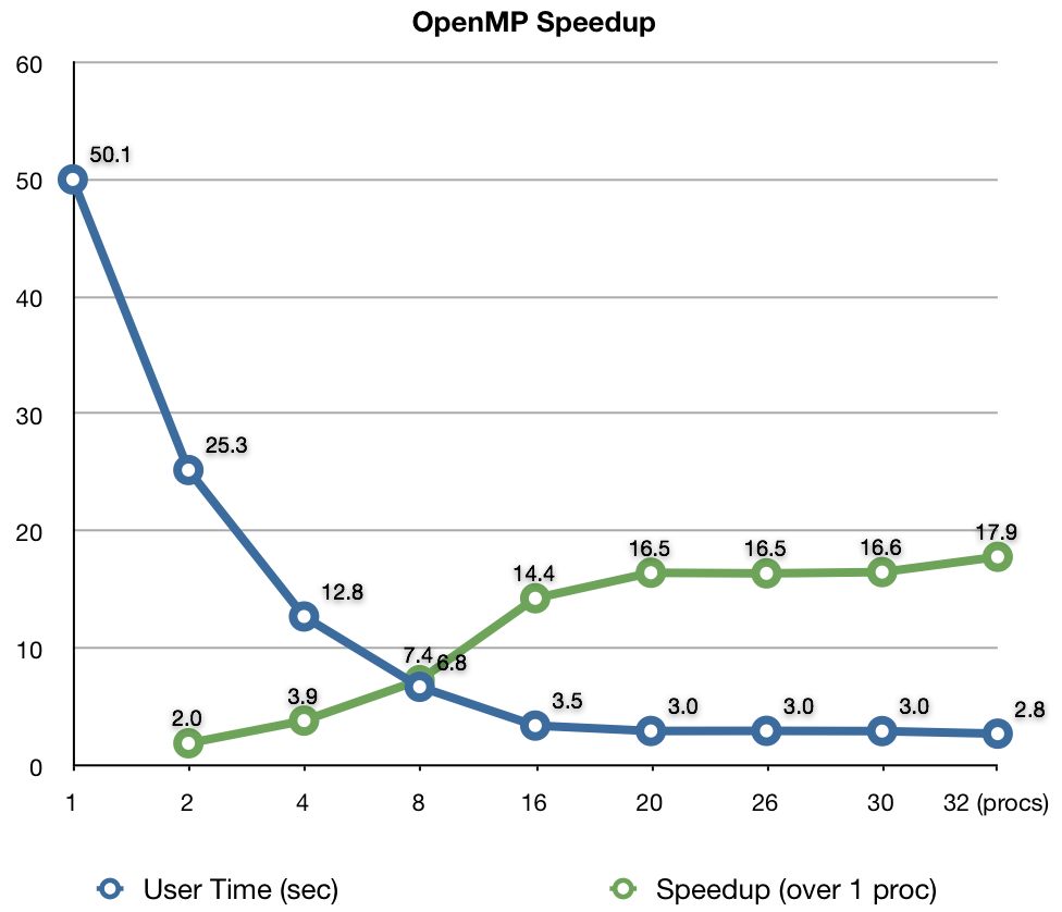
The graph above shows the speedup that a few OpenMP statements can give with very little effort. OpenMP is a simple way to parallelize a C/C++ program which allows you to run a program on many processors at once. However, unlike MPI which can run on many different machines (like a cluster), OpenMP can only be run on one computer at a time. Since most new machines have multiple processors (or cores), OpenMP is quite useful.
I've added a couple dozen OpenMP statements to the code I'm working on. The blue line shows how long (in seconds) it took me to run a test problem on between one and 32 processors. The green line shows the speedup compared to running on a single processor as a ratio of time. It is very typical of parallel programs that the speedup isn't linear and flattens out at high thread count. This small test problem deviates at 16 processors; when I do a real run (which will be much larger and the parallelization more efficient) I may see nearly linear speedups all the way to 32 processors.
I think it's pretty neat how with very little effort I was able to significantly speedup my code.
more ...Monte-Carlo Whoopass
Don't worry about the physical meaning of the two plots below:
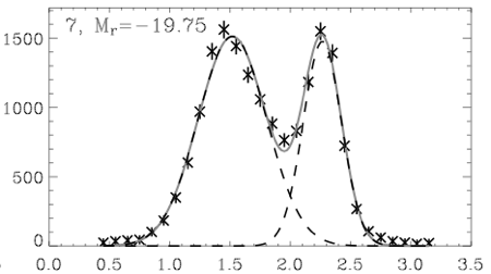
Taken from Baldry et. al. (2004),figure 3 (plot 7).
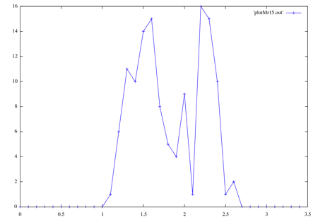
My plot of entirely fake data that means almost nothing.
Just notice that the two peaks are pretty much in the same places on both graphs, 1.5 and 2.2. The first graph shows physical data (stars) and a double-Gaussian fit (light solid line). The second graph is the result of my using Monte-Carlo fitting to make entirely fake data using the first curve. The real graph has over 10,000 items to make that smooth distribution, while with only about 100 items Monte-Carlo is already starting to look like the real thing. Of course, it will take much more items to capture the smoothness and the "long-tail" on each end.
I just wanted to share because the whole thing I wrote, which includes a simple function integration (for normalization), worked on my first try.
more ...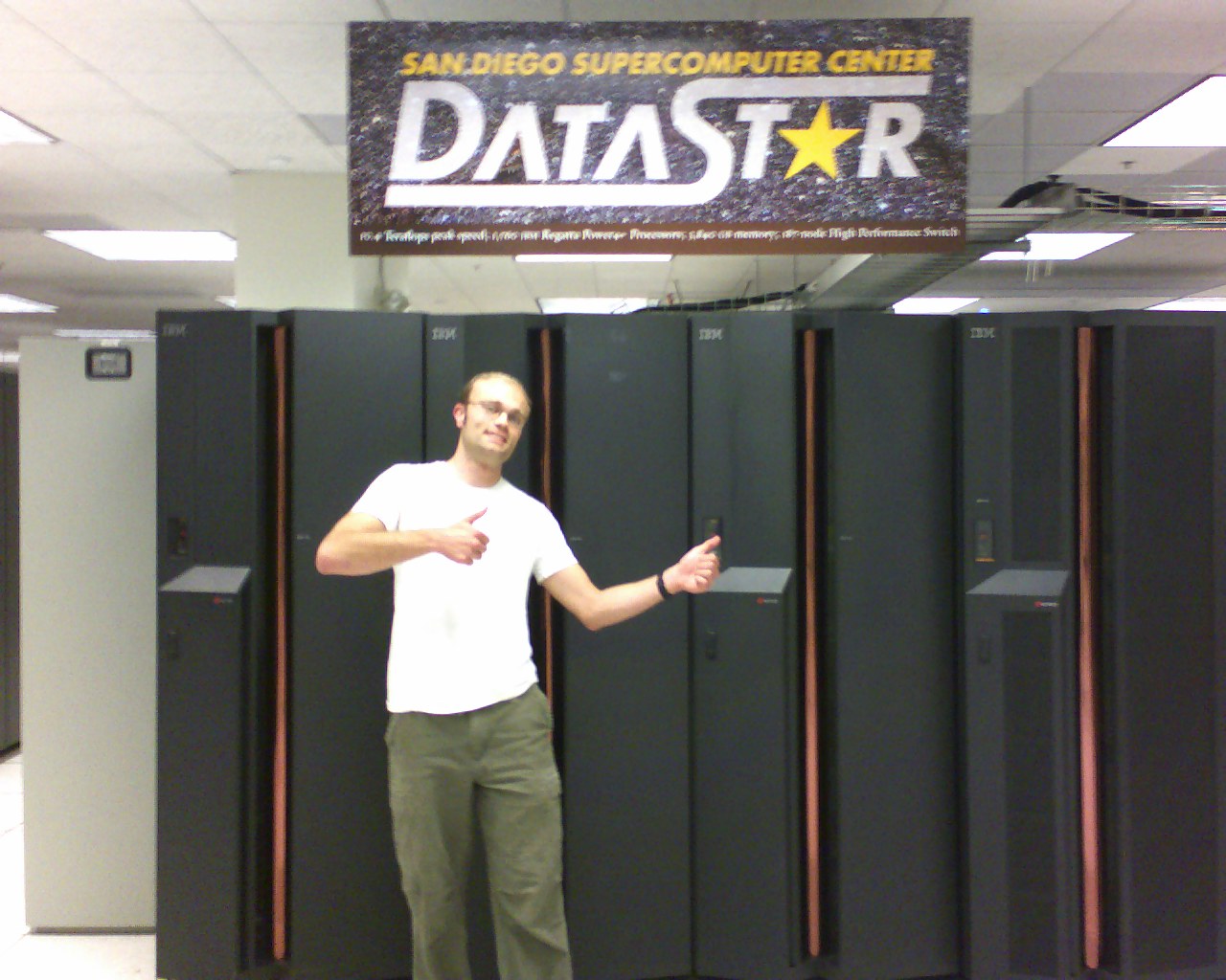
A Bit of Shiny
Below is a little animation that I made yesterday that shows what I have been doing lately. The green dots correspond to the positions of dark matter particles, while the little yellow squares are the locations of dark matter haloes that I'm interested in. The white lines are the edges of the simulation volume, and you can see the axes triad in the bottom-left corner. To give you an idea of the scale of what's depicted here, each edge of the cube is 50 Mpc, or 163 million light years. Our entire galaxy is only about 20 kpc or 65,000 light years across.
In the first part of the movie, the cube is rotated about its center. Next, while looking along the z-axis, the volume of the cube plotted is reduced until only 1/10th of the cube is shown. Then, this 1/10th thickness is scanned through the entire cube, and then the volume plotted is replenished back to full.
The things to notice are how the dark matter form areas of high density, which are connected by filaments. Between these are areas of relatively few particles, which are called voids. This is how our universe really looks, with huge collections of galaxies clustered together, separated by huge expanses of nearly empty space. I should point out that there are many more galaxy haloes in this box besides the yellow boxes.
What I was looking for was one of those yellow boxes which is fairly isolated from areas of high density dark matter. I picked one, and now I am doing this same simulation again, but with higher resolution boxes centered on the area of interest. The simulations I'm doing right now are fairly cheap (in computer time currency). I want to be sure that when I run big, time-intensive simulations in the future that I've picked a good area to focus my attention on.
I did this visualization with Visit, a stereo, 4D visualization tool out of the Livermore National Lab. The "stereo" means that it can create two images of the same data that are slightly offset, which create a 3D effect if viewed correctly. The fourth dimension is for time, as it can handle time-ordered data sets. I then used Visit's Python scripting features to output 800 individual PNGs, which I then stitched together (exactly like my time lapse movies) to make this movie.
more ...Galaxy Family Tree
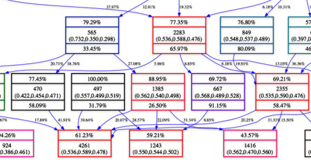
Above is a part of what I've been working on lately. It's a small part of the galaxy family tree that I've derived from a large simulation. In the simulation there are several ingredients that are thrown in the "box." Relevant to this are the dark matter particles, which coalesce into consituents of galaxies. The dark matter particles have unique id numbers. Using a some code I didn't write, I process the simulation data and make a list of galaxies along with the particles in each galaxy. Then, using some code I did write, I track particles and galaxies over a number of time steps, which builds a relational mapping. Then, I use Graphviz to make a nice tree, as you see above.
Inside each box are either three or four data values. The top grid shows what percentage of the particles in that group came from no group, the middle grid shows both the number of dark matter particles that are in the group and the position of the group, while the bottom grid shows the percentage of the particles that go to no group. The simulation takes place inside of a 3D box with length 1 on a side and periodic boundaries (which means the distance between 0.9 and 0.1 is 0.2, not 0.8). The colors of the box correspond to its ranking in size, red is the largest, green the smallest. The numbers next to the arrows are what percentage of the parent group goes to the child group.
The goal of this is to get an idea of how the galaxies form over the course of the simulation. Of course the simulation tries to mirror reality, so this family tree may be worth something.
more ...My Research
For the better part of half a year now I've been working slowly on a project with Mike Norman, my advisor. I'm basically implementing a test of the efficiency & accuracy of the cosmological simulation code his group uses. I do this by sticking a ring of gas into the simulator and watching the gas spread out. I compare the computer simulation to how it should go if all things were perfect (which the simulation is not). The two plots below are a culmination of my accelerating efforts.
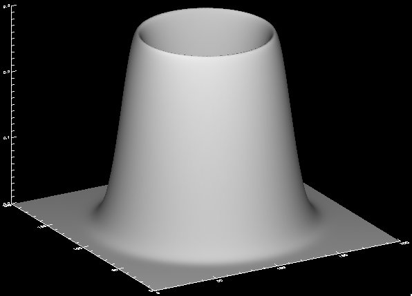
Above is a 3D plot of the gas density. The two horizontal coordinates are the x-y position, while the vertical gives the density at that point. I'm doing my simulation in two dimensions right now, eventually I'll go to three.
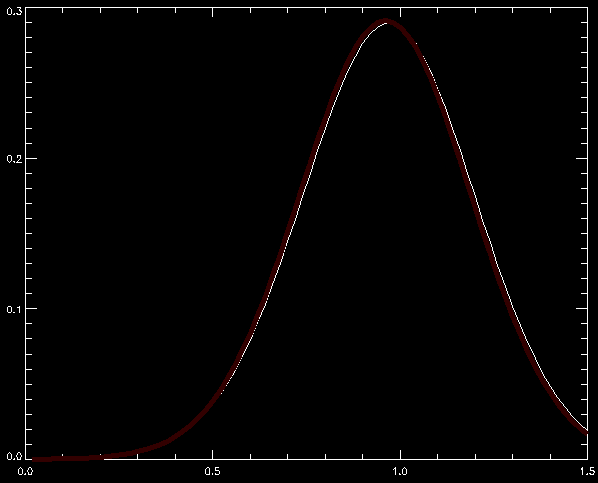
The white line above (hidden by the red line) is a sideways slice of the density, starting at the center going out. The red line is a best curve fit of the white line. The curve fit is very good because the white line was generated by the same function I'm using for the best fit, but the picture shows my fitting technique works, and that's what matters.
I hope to make further, faster progress! I'll post things here as I go along.
more ...